Index
- ODE Description of a Second Order System
- [[#definition-of-as-is-hs-a_dc—zeta—omega_0|Definition of , , , , , ]]
- Dynamic Behaviour of a Second Order System (Modes of Poles)
- Frequency Analysis of Complex Poles for Second Order System
Okay at this point we can go and discuss and recall what happens for a second order system.
ODE Description of a Second Order System
 So we take a second order system by writing a second order dynamic model.
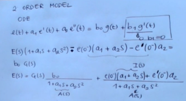
So we start from the ODE which is the ordinary differential equation which represents this kind of systems, in time domain:
And I take the simple model where I consider to have this term equal to .
I don’t have any zeros in the transfer function.
Okay so we restrict the study to this simple model we go to the Laplace domain.
So I can write:
And I take this polynomial here:
So we take a second order system by writing a second order dynamic model.
So we start from the ODE which is the ordinary differential equation which represents this kind of systems, in time domain:
And I take the simple model where I consider to have this term equal to .
I don’t have any zeros in the transfer function.
Okay so we restrict the study to this simple model we go to the Laplace domain.
So I can write:
And I take this polynomial here:
Definition of , , , , ,
==Then you define two polynomials: which defines the pole of the system, and a polynomial depending on the initial conditions==.
So we can write :
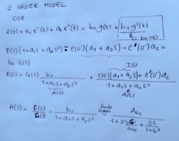 == is a transfer function, which gives me the ratio between the output and the input==, when the initial condition is (a step function):
So we have the dynamic of the system which is defined by 3 parameters:
== is a transfer function, which gives me the ratio between the output and the input==, when the initial condition is (a step function):
So we have the dynamic of the system which is defined by 3 parameters:
- Gain in DC (Direct Current, meaning at low frequency)
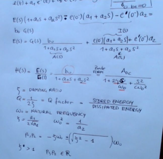
- : damping ratio, also defined by (the factor)
- : natural frequency
We have that is the damping ratio, ==an alternative way to express these behavior here is the factor which essentially describes the stored energy or power divided by the dissipated energy==. And then we have which is the natural frequency. Obviously we have that is: … Okay, the two poles , , are: …
Dynamic Behaviour of a Second Order System (Modes of Poles)
 So we have obviously two cases which result into a different dynamic behavior.
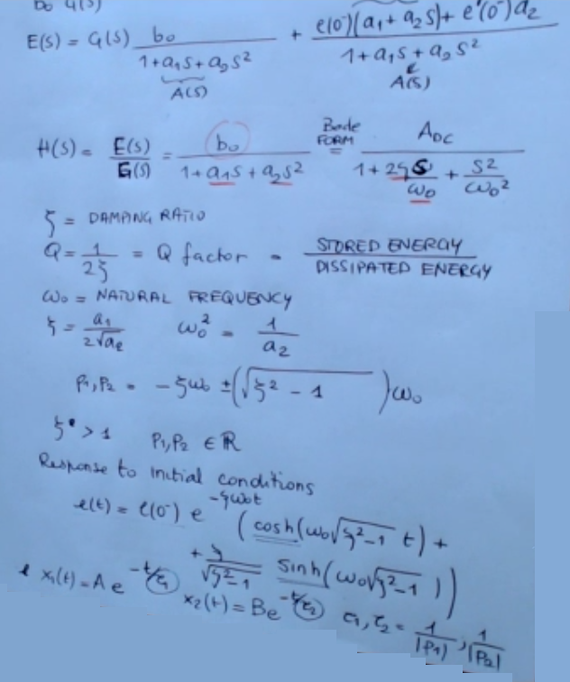
==The first is if this parameter damping ratio is larger than (so if ), and in this case the two poles belongs to the real numbers and in this case we can write for instance the response to the initial conditions of the system, in this way==:
Actually this is here you see you have cause hyperbolic cosine which actually means that this function here is a combination of the two exponential functions: and
And this two parameter and are simply: …
So actually even if this formula here gives an expression which resembles the sum of cosine and sine it’s a dipol function so they are obtained by combining the exponential functions with two exponential functions.
Obviously in case of response to a step function we have a behavior which is the similar:
So we have obviously two cases which result into a different dynamic behavior.
==The first is if this parameter damping ratio is larger than (so if ), and in this case the two poles belongs to the real numbers and in this case we can write for instance the response to the initial conditions of the system, in this way==:
Actually this is here you see you have cause hyperbolic cosine which actually means that this function here is a combination of the two exponential functions: and
And this two parameter and are simply: …
So actually even if this formula here gives an expression which resembles the sum of cosine and sine it’s a dipol function so they are obtained by combining the exponential functions with two exponential functions.
Obviously in case of response to a step function we have a behavior which is the similar:
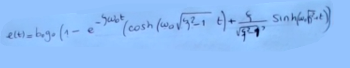
And then same as before, I’m going forward and I write it:
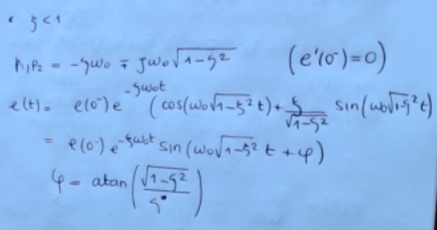
==This is what happens if we have the opposite situation that is where : so , belongs to the complex numbers== and we can write them this way: … So in that case we have the response to that initial condition:
Where is the inverse tangent of …
Obviously all these responsible initial condition I have written are under the assumption of having the first derivative initial condition equal to (when defining the 2 order model we have supposed ), which I have to take in account.
So we have the resposne to a step funciton, as usual:
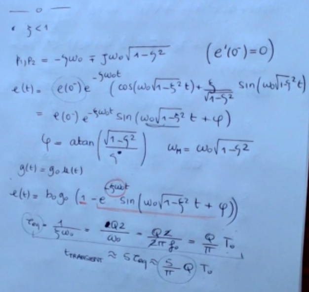 is the same, defined before.
What we can say here we see that we have a decay of these transient response here ().
The steady state is represented by this one here:
So the equivalent time constant is:
We can also also express it in terms of , is the same: …
So for instance and at the end, we can write: …
is the period of the natural frequency.
Actually you see that the frequency of the transient response this part here is not exactly the natural frequency, we have this modal frequency which is given by this one, nd this is tell us how long is the time needed for the transient to vanish:
is the same, defined before.
What we can say here we see that we have a decay of these transient response here ().
The steady state is represented by this one here:
So the equivalent time constant is:
We can also also express it in terms of , is the same: …
So for instance and at the end, we can write: …
is the period of the natural frequency.
Actually you see that the frequency of the transient response this part here is not exactly the natural frequency, we have this modal frequency which is given by this one, nd this is tell us how long is the time needed for the transient to vanish:
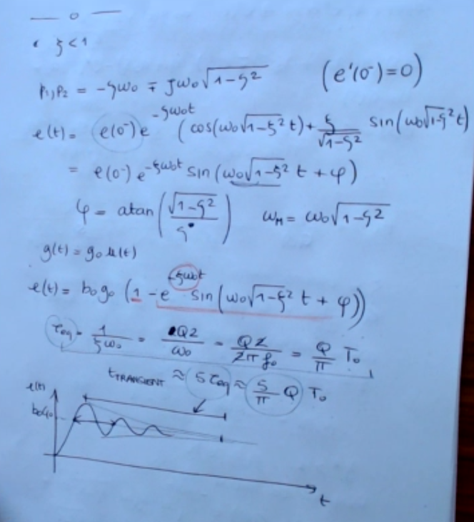 So we can think about the rule of thumb which is also the number of periods you have of the natural frequency you have to wait before the transient vanishes.
So obviously this corresponds to having this value here, this time this is and length of this transient here is described by this parameter.
Whereas this is given by something which resembles this frequency here.
So we can think about the rule of thumb which is also the number of periods you have of the natural frequency you have to wait before the transient vanishes.
So obviously this corresponds to having this value here, this time this is and length of this transient here is described by this parameter.
Whereas this is given by something which resembles this frequency here.
Frequency Analysis of Complex Poles for Second Order System
Now we go to the frequency domain, in case of two complex poles:
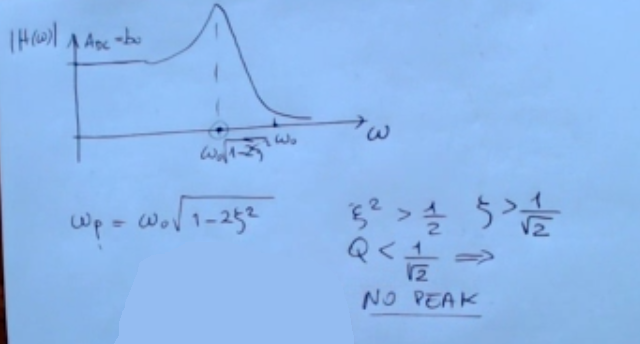 We put here and here this, we start from .
==We have two zeros so this is a DC coupled system.==
So we have a peak which is at a radian frequency close to , and this is the exact frequency of the peak, obviously if this larger than that means that:
Which corresponds to:
Then this peak is not more present.
So no resonant frequency.
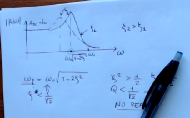
So this peak here and this frequency exists only if we have this condition satisfied:
We put here and here this, we start from .
==We have two zeros so this is a DC coupled system.==
So we have a peak which is at a radian frequency close to , and this is the exact frequency of the peak, obviously if this larger than that means that:
Which corresponds to:
Then this peak is not more present.
So no resonant frequency.
So this peak here and this frequency exists only if we have this condition satisfied:
 The name of the peak is “resonant frequency”, is the maximum response to an input.
But this frequency here we have the maximum possible response to a harmonic input.
And so if I draw this two curves:
The name of the peak is “resonant frequency”, is the maximum response to an input.
But this frequency here we have the maximum possible response to a harmonic input.
And so if I draw this two curves: