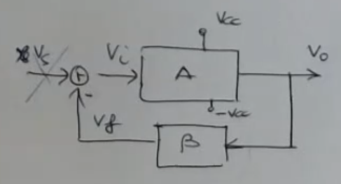
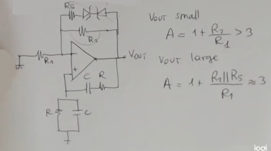
I need a (preferably) marginally stable output, so: 1+β(jω)A(jω)=0
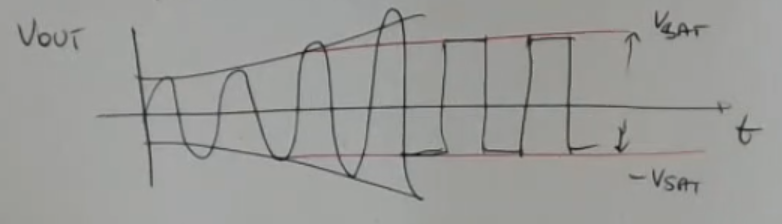
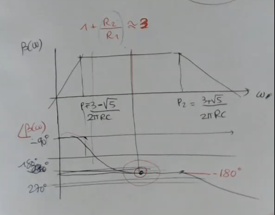
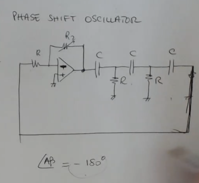
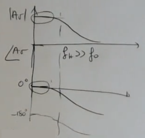
Solution: “Barkausen conditions”:∣βA∣≥1∠βA=180°(If ∣βA∣ is exactly 1, we will have a marginally stable output)
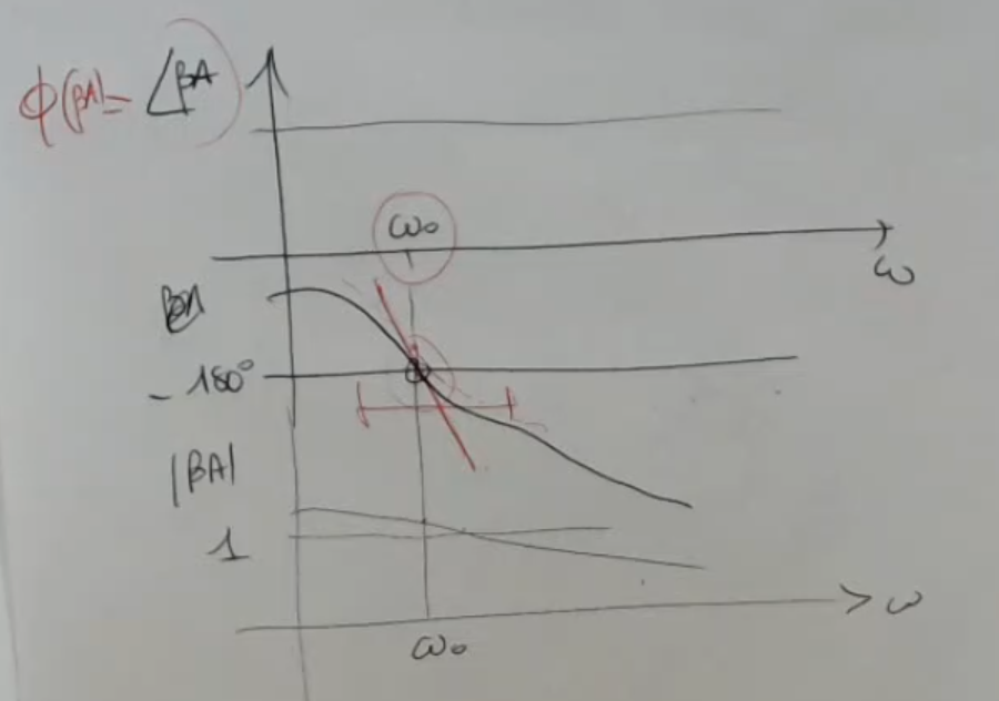
Frequency stability: the two parameters (β and A), which are the gain of the amplifier and the gain of the feedback network, have to be stable in time, not changing. ⇒ We can “take a big slope” when crossing the −180° degrees line, so around ω0 (where I need to oscillate).
Frequency of an FM modulated signal:f(t)=f0(1+f0fAx(t))
FM modulation using an integrator: (For instance if I have x(t) which is a slowly growing invariant signal, then the frequency would increase a litte over time.)
Bandwidth of the FM modulated signal: Where:
ΔfMAX=fA⋅xMAX.
And fA comes from: f(t)=f0+fAx(t).
Since FM transforms a the physical input variation into a variation of frequency, it is a very robust solution to reject noise.
Complete FM Circuit:
The sensor is part of the oscillator.
The FM Demodulator gives as output a voltage related to the frequency in input.
Real World Measures:
FM is used for signals which can be static but also they have a large bandwidth up to 100kHz
The typical value for f0 is 2MHz (much larger than the maximum signal frequency).
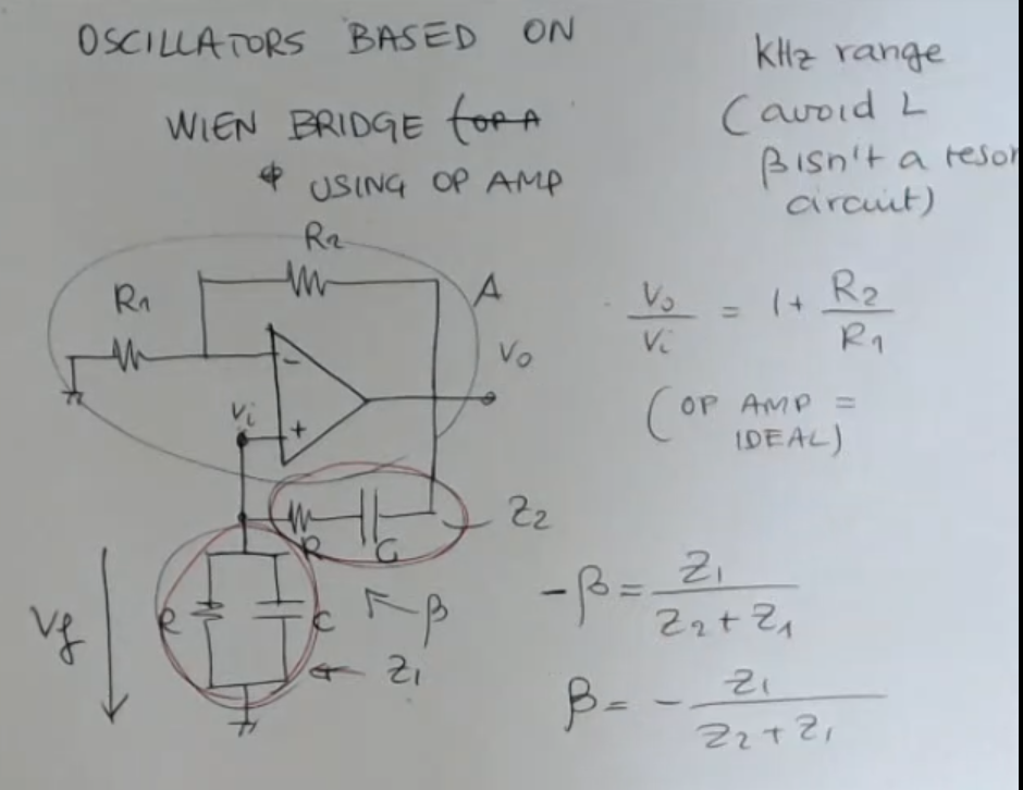
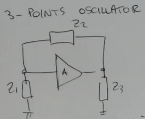
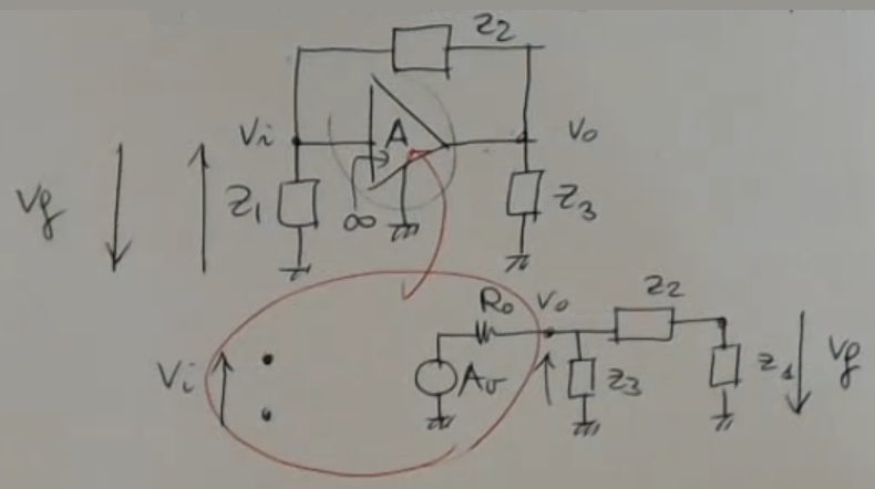
For f≪fh we have that*:A=AvjR0(X3+X1+X2)+jX3(jX1+jX2)jX3(jX1+jX2)If we impose X1+X2+X3=0, or more in general:Xi+Xj=−XzWe will find: A=Av
Hartely oscillator: 2inductances and 1capacitance.
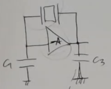
Colpits oscillator: 2capacitances and 1inductances.
Using an AT-cut quartz in a Colpits oscillator: (This circuit will oscillate only at frequency in which the quartz acts as an inductance, so for f0 in the interval [ωs,ωp])
Q-factor value: (Adding a capacitance in series or in parallel to our quartz, will reduce this value, not goood)Q=ωsReqCeq1
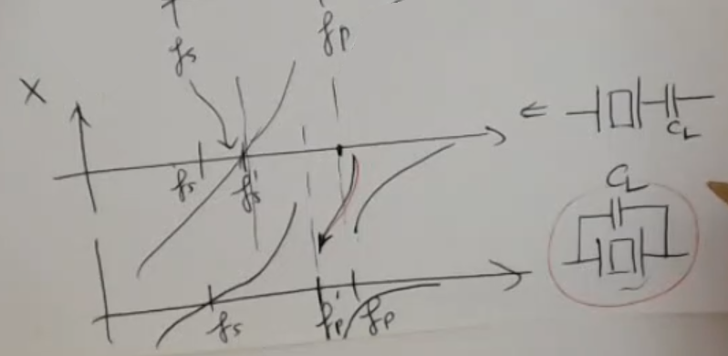
Adding a capacitance in series or in parallel to the quartz: (Adding a capacitance in series or in parallel can reduce the frequencies fs and fp, giving us more control, good)
Special frequencies: (They depend on the type of cut of the quartz)ωs=LeqCeq1ωp=CELeqCeqCE+Ceq
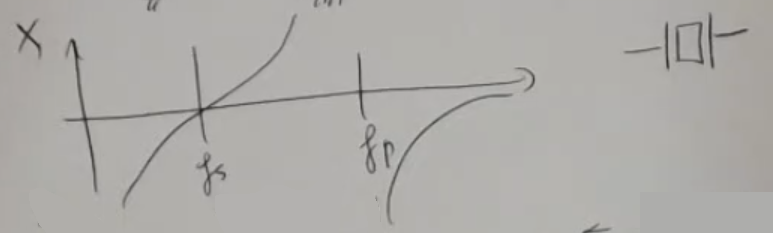
Reactance formula (Xeq:Zeq=jXeq):Xeq=−ωCE11−ωp2ω21−ωs2ω2
Plot of 1−ωp2ω21−ωs2ω2:
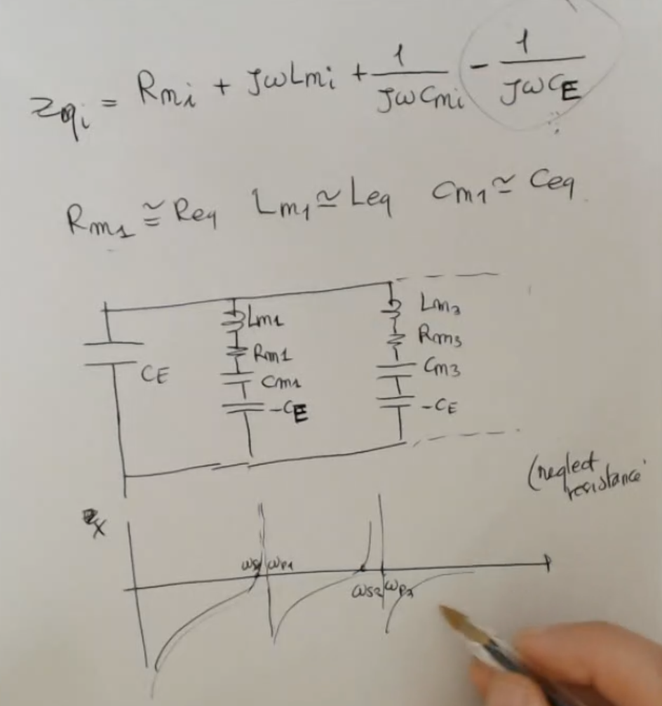
More realistic impedance model: (If we work at a high frequency (f∈[20MHz÷30MHz]), we need to consider this additional impedaces, after the first). (If we work at lower frequencies (<10MHz) we can consider just the first Zeq).
Formula for each component:Lmi=81k2d2mCmi=(i⋅π)28kd2Rmi=8(i⋅π)2k2d2λAnd the value of ωsi:ωsi≈i⋅ws1
Real World Measures:
At ω=10MHz, we gave some common values for the AT-cut quartz’s impedances:Leq=100mHCeq=15fFReq=20\ohm
Terminology:
m,λ,k : mass, dumping coefficient, elastic coefficient of the piezoelectric slice.
ZM : mechanical impedance of the medium, as an example when we talked about the ultrasonic transducer we said that it used an “added damper”, in that case ZM would represent this added dumper.
/../../Notes--and--Images/Pasted-image-20230921232009.png)
/../../Notes--and--Images/Pasted-image-20230719105215---Copia-1.png)
/../../Notes--and--Images/Pasted-image-20230719105145-1.png)
/../../Notes--and--Images/Pasted-image-20230719105202.png)
/../../Notes--and--Images/Pasted-image-20230719105215.png)
/../../Notes--and--Images/Pasted-image-20230719105223-1.png)
/../../Notes--and--Images/Pasted-image-20230719105232-1.png)

/../../Notes--and--Images/Pasted-image-20230720170012-1.png)
/../../Notes--and--Images/Pasted-image-20230720165950-1.png)