SaM - Charge Output Accelerometer

Remeber:

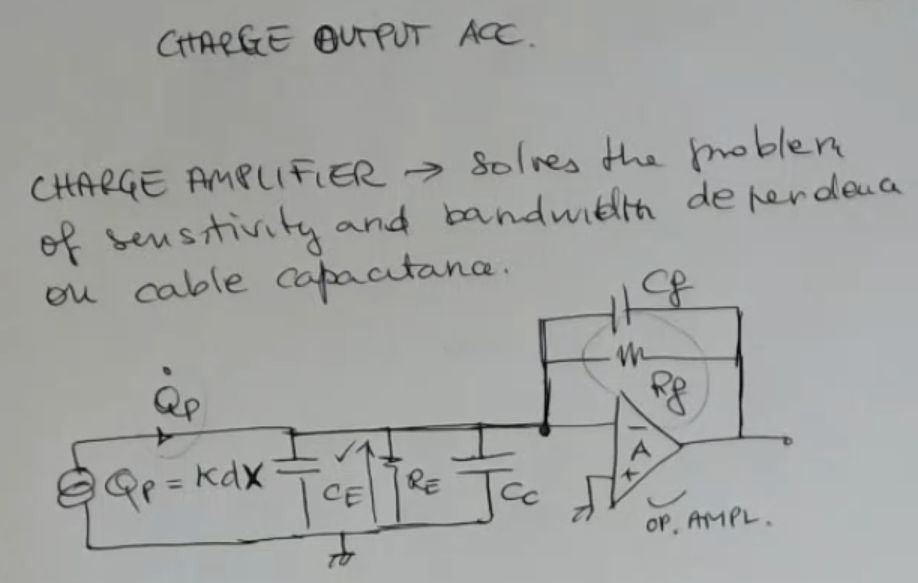
So as we have seen, for piezo-accelerometer the output depends on the cable capacitance. To solve this problem we can change the topology of the front end circuit and in particular the idea is to use a charge amplifier:

• So the charge amplifier solves the problem of sensitivity and bandwidth dependence on cable capacitance.
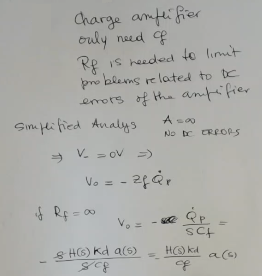
• $R_f$ is placed here as needed in order to limit, the problems of offset related to the DC errors of the amplifier.
• Another reason for having $R_f$ is the biasing current, without $R_f$ the biasing current will constantly charge $C_f$.

If we consider the amplifier ideal, so $A=\infty$ and no DC errors, the output will be:$\frac{V_0(s)}{a(s)}=-\frac{K\cdot d}{C_f}H(s)$Where $H(s)$ is the same for all accelerometers:$H(s)=\frac{m_S}{m_{S}s+\lambda +\frac{k}{s}}$ The sensitivity of the complete systems (sensor + amplifier) is: ${\alpha }_0=\frac{K\cdot d}{C_f}\frac{m_S}{k}$

Instead if we consider that the gain of the amplifier has the form $A(s)=\frac{A_{DC}}{1+\frac{s}{{\omega }_H}}$Then it’s like having this case:

• $C_T=C_E+C_C$
  • $C_C$ was the capcaitance realted to the cable.
    ~Ex.: take for instance for $10$ meters of cable, which result in a $1nF$ capacitance which is really a large value.
    But if you divide this value here for the gain of the amplifier (and if the amplifier is selected correctly this value is very high), then you reduce this capacitance, and you are able to neglect the presence of the cables.
• So for $A{R}_E\gg R_f\&\frac{C_T}{A}\ll C_f$We can use the simple formula:${\lim }_{\omega \to \infty }\frac{V_0}{a}=-\frac{K\cdot d}{C_f}H(\omega )$

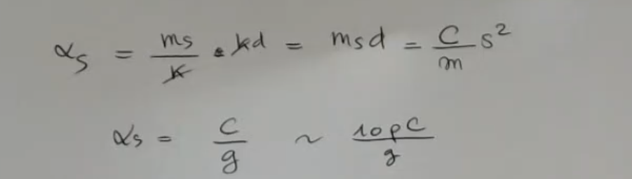
Some real values, for charge output accelerometer:

• $\frac{1}{R_f{C}_f}\approx 0.1\text{Hz}$.
• ${\alpha }_S\simeq 10\frac{\text{pC}}{\text{g}}$ (pico-Coulomb per $g=9.8\frac{\text{m}}{s^2}$ the constant of gravity).
  Where ${\alpha }_S=m_S\cdot d$ is the sensitivity related only to ???TODONOT_SURE_ABOUT_THIS

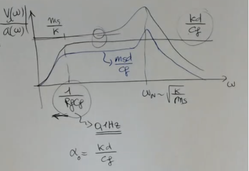
Here is the bode plot:

---

• And you have to change the type of front end because it should be avoided this dependence of the sensitivity and of the bandwidth of the sensor on the cables, obviously.
• And this is simply done by changing the topology of the front end circuit and in particular the idea is to use a charge amplifier.
  ⇒ So the charge amplifier solves the problem of sensitivity and bandwidth dependence on cable capacitance.
• With the addition of this amplifier, we impose that the voltage drop across all resistances and capacitance $C_E$, $R_E$, and $C_C$ is $0$, doing this all the current ${\dot{Q}}_P$ (created by the piezoelectric effect) can flow into $Z_f=C_f\parallel R_f$.
• So instead of amplifying the voltage output of the sensor, we amplify the current of the sensor.

Calculating:

• Another reason for having $R_f$ is the biasing current, without $R_f$ the biasing current will constantly charge $C_f$, capping the value of the output at $V_{cc}$ after a certain period of time.
  So $R_f$ is placed here as needed in order to limit, the problems of offset related to the DC errors of the amplifier

So first of all we perform a very simplified analysis, simply find analysis:

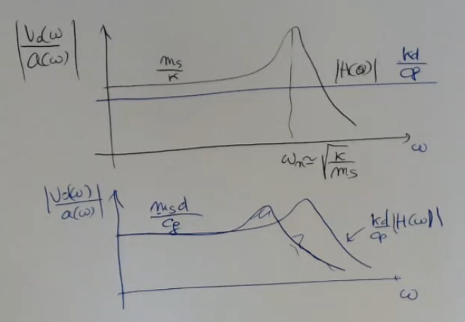
• First plot represent $H(s)$ (unchanged from the previous lesson), and the output without $H(s)$, we need to multiply the two to find the total response system, and we do so in the second plot.
• This time tho $C_F$ doesn’t depend on the cable, it is something which belongs to the front end amplifier, and I decide its fixed value.
• Moreover from this very simplified analysis, we see that we have a DC coupling.
  ⇒ So everything that comes from the sensor is transferred also at low frequencies.
  But we know it is not so because we know that the sensor itself is not able to sense DC accelerations, saddly this sensor is not able to perform static measurements.
• I have neglected something which is really important, I have considered ideal the amplifier, instead we can start and look what happens.

We can start to consider some of the non-idealities of the amplifier:

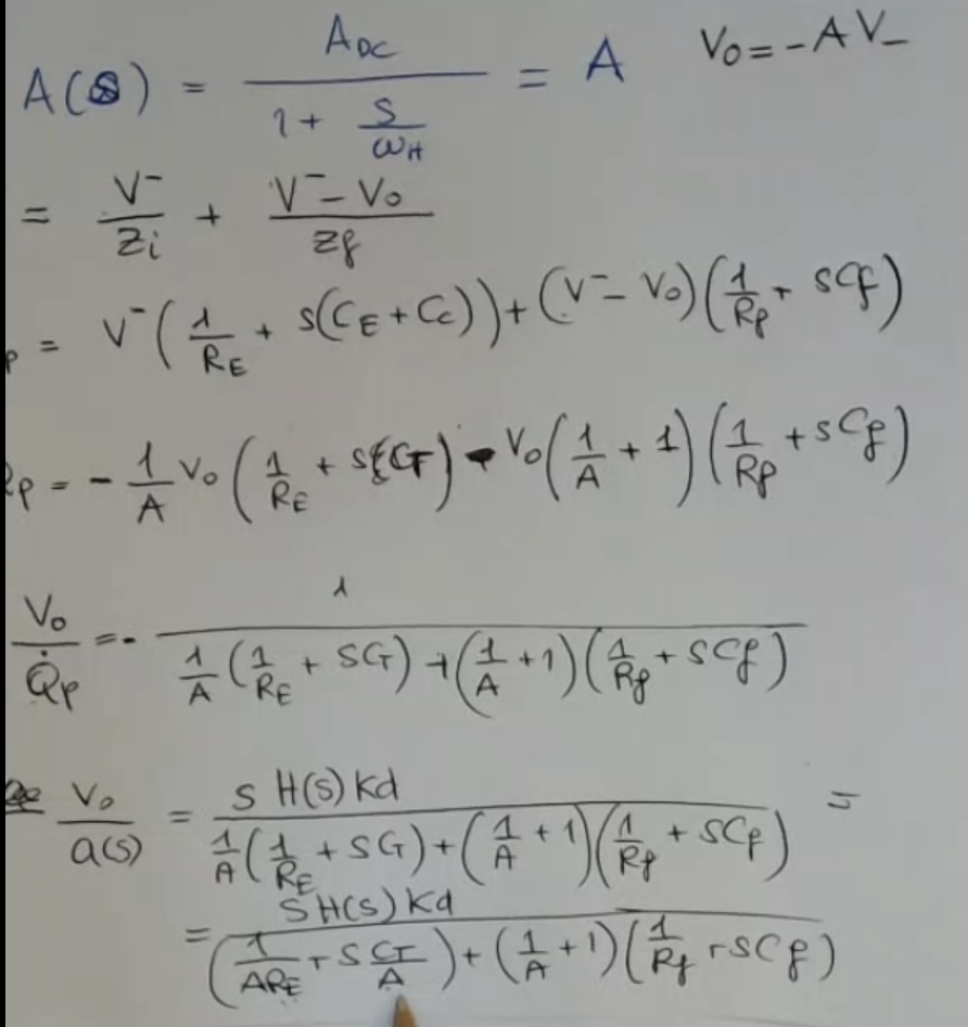
• $A(s)$ : actual gain of the amplifier.
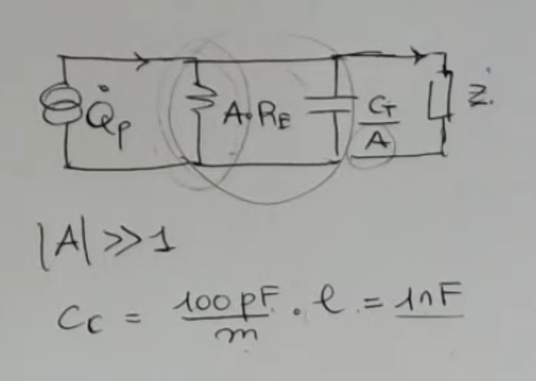
• We see after some calculation that $\frac{V_o}{a(s)}$ is more complicated than before, and actually it still depends on the parasitic and cable capacitances ($R_E$, $C_E$, $C_C$)
• $C_T=C_E+C_C$
• Still you have a very good effect by using this front end topology, because it’s like having a really large resistance and a very small capacitance, for a large value of $A$.

So it’s like having this case:

• $C_T=C_E+C_C$
• $C_C$ was the capcaitance realted to the cable, and for instance for $10$ meters of cables we have a $1nF$ capacitance which is really a large value.
  But if you divide this value here for the gain of the amplifier which if the amplifier is selected correctly is very high then you reduce this capacitance, and you are able to neglect the presence of the cables.
• I have incapsulated the amplifier in the values of the parasitic components.

Okay, so we go back to this part here:

• So for $A{R}_E\gg R_F\&\frac{C_T}{A}\ll C_f$We can use the simple formula:${\lim }_{\omega \to \infty }\frac{V_0}{a}=-\frac{K\cdot d}{C_f}H(\omega )$
• NOTE: The professor sais $a_0$ it should be $a$.

Plot:

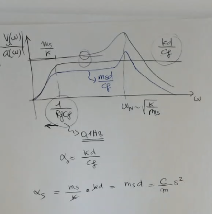
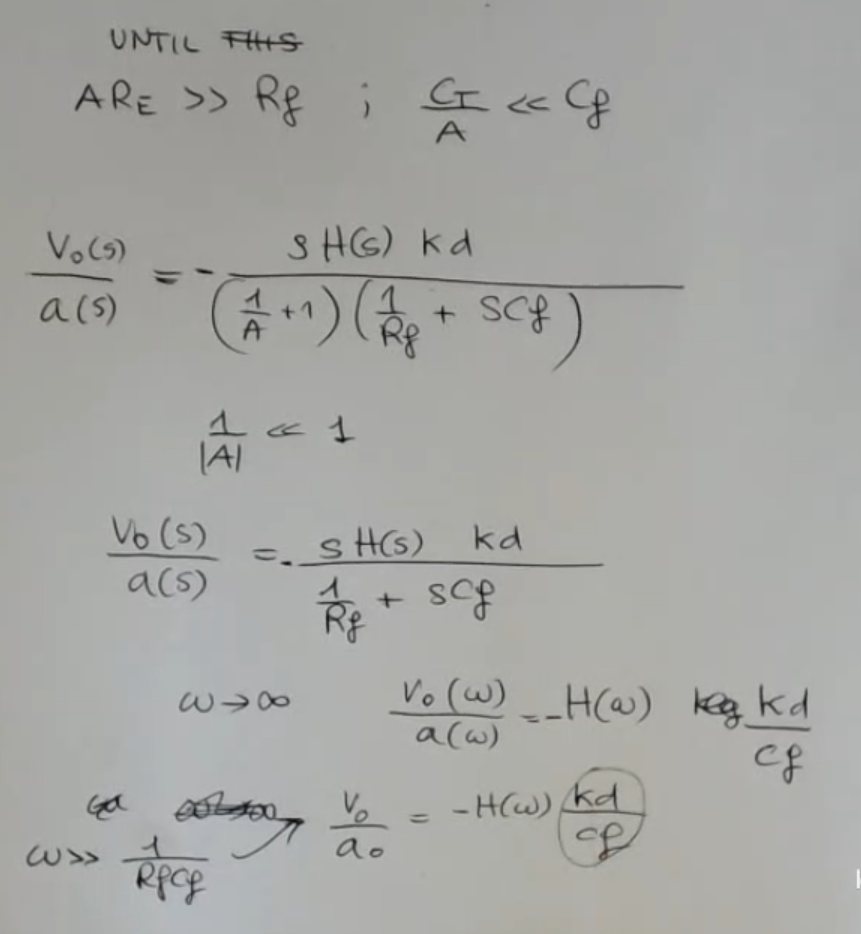
• So we will have a zero in $0$, and then a pole at $\frac{1}{R_f{C}_f}$, but this time the value of this pole is “arbitrarly small” (not really).
• Remeber that we can’t select a too large value of $R_f$, since $R_f$ has to limit the effect of the DC errors of the amplifier, if it is too large it will not do its job.
• The important is that the gain and bandwidth do not depend on the cable but only on the value of components intentionally placed in the feedback network.
• So we have good performances.
• Pay attention, ${\alpha }_0$ is not just the sensitivity of the sensor, ==it is the sensitivity of the sensor $+$ the amplifier==, it depends on $\frac{1}{C_f}$, so it depends on the amplifier which is not integrated with the sensor.
• ${\alpha }_s$ should be the sensitivity of the simple mechanical parts of the sensor.NOT_SURE_ABOUT_THIS

Often you find ${\alpha }_s$ expressed as coulomb divided by $g$.