CDS - Topic of Choice 'Bifurcations'

What is a Bifurcation?

Let’s consider a non-linear system $f$ that also depends on some parameter $k$, so:$\dot{x}=f(x,k)$We have that the system equations depends on the parameter $k$, so:

• The steady states, their existance, the Jacobian matrix of the linearized system, as well as the stability of the steady states, can all depend on this parameter $k$.

---

If the system $f$ has a flow that does not change with the parameter $k$, then we say that the system is structurally stabile, in more details we say that:

A system is structurally stable if the flow in the phase space does not vary when the system’s parameters change.

• The structural stabilty is related to the stability of the steady states: if all steady states are hyperbolic, then the system is structurally stable.
• A change in the geometry of the phase space may occur only when a steady state is non-hyperbolic:
  • ~Ex.: steady states that disappear when changing the parameter.
  • ==To have structural instability we need that chagning the parameter we change the sing of the eigenvalues==, so for a certain value of the parameter, we have a change of sing, so for $k^{\ast }:{\lambda }_1\text{ or }{\lambda }_2=0$, we say that we have a “bifurcation” ($k$ is the parameter)

---

A steady state $x^{\ast }$ such that $J(x^{\ast })$ (the Jacobian Matrix) has no null nor purely imaginary eigenvalues is said hyperbolic.

And if we have an hyperbolic steady state from the Hartman-Grobman Theorem, we can say that: If $x^{\ast }$ is hyperbolic, then there is a ==homeomorphism== defined in some neighborhood of $x^{\ast }$ in ${\mathbb{R}}^n$ locally taking orbits of the nonlinear flow to those of the linear flow. The homeomorphism preserves the sense of orbits and parametrization by time.

Also near an hyperbolic steady state the geometry of the phase space is preseved by the linearization.

---

(My Notes / My Take / My Thoughts, TAKE THEM WITH A GRAIN OF SALT!) (Under this section you’ll find the professor’s notes.)

Let $x^{\ast }$ a steady state of the non-linear, monodimensional system $\dot{x}=f(x)$, then $f(x^{\ast })=0$.

1. If we perform the Taylor Series around $x^{\ast }$ we will obtain:$\dot{x}=f(x^{\ast })+f^{\prime }(x^{\ast })(x-x^{\ast })+O(x^2)$Where:
   • $f(x^{\ast })=0$
   • $f^{\prime }(x^{\ast })\in \mathbb{R}$, we can also call it $a$.
   • $O(x^2)=0$, (we ignore it)
2. We define a new system (transposed) near the steady state, so: $y(t)=x(t)-x^{\ast }$, such that $\dot{y}=\dot{x}$, and we can define the linearized system by substituting to the Taylor series as:$\dot{y}=f^{\prime }(x^{\ast })y\text{or}y=ay$
3. So we can find the solution of the linearized system $(\dot{y}=ay)$ preatty easly:$y(t)=y(0)e^{at}$
4. Notice how:
   • If $a>0$, so if we have $f^{\prime }(x)>0$, then this linearized system will diverge.
   • While if $a<0$ (meaning $f^{\prime }(x)<0$) it will converge.
5. For higher-dimensions systems, we will see that $f^{\prime }(x^{\ast })$ becomes a matrix, more specifically the Jacobian Matrix, and we will analyze like we did for linear systems its eigenvalues.

(Professor’s Notes)

The linearization is a method for characterizing locally the geometry of the phase space (flow), locally meaning in the neighborhood of $x^{\ast }$.

Let $x^{\ast }$ a steady state of the non-linear system $\dot{x}=f(x)$, then $f(x^{\ast })=0$. Let $\eta$ be a perturbation of the steady state $x^{\ast }$. We want to study the “perturbated solution” $x(t)=x^{\ast }+\eta$.

1. From: $x(t)=x^{\ast }+\eta$ we can say that $\eta =x(t)-x^{\ast }$.
2. And if we derive both part in time, we have that: $\dot{\eta }=\dot{x}=f(x)$
3. If we expand the $f(x)$ with Taylor, near $x^{\ast }$, we have:$\dot{x}=f(x^{\ast })+f^{\prime }(x^{\ast })(x-x^{\ast })+O(x^2)$Where:
   • $f(x^{\ast })=0$.
   • $\eta =x(t)-x^{\ast }$
4. Finally we have that $\dot{\eta }=f^{\prime }(x^{\ast })\eta$, then if we study this “linearized system”, and we see that $\eta$ grows, meaning for $f^{\prime }(x^{\ast })>0$, then we have that the original system will diverge from the steady state $x^{\ast }$, meaning that $x^{\ast }$ is an unstable steady state.
   While if we have that $f^{\prime }(x^{\ast })<0$ then this $\eta$ will go toward zero, meaning that the perturbated system will converge to the steady state, $x^{\ast }$ is a stable steady state.
   However if $f^{\prime }(x^{\ast })=0$ we cannot say anything about the original system $f(x)$.

Given a system:$\dot{x}=f(x)$And a steady steate $x^{\ast }$ of this system, if this steady state is hyperbolic then we can study the stability of the linearized system: $f^{\prime }(x)=\frac{d}{dx}f(x)$And its stability or instabilty will be the same as the original $f(x)$ system. ==However if $f^{\prime }(x)$ is marginally stable, then we cannot say anything on the stability of $f(x)$==.

---

So given a structurally unstable system $f(x,k)$, we can define:

• Definition ‘Bifurcation’:
  A bifurcation is a drastic change of the flow of a dynamic system, occurring when some parameters $(k)$ change.
• Definition ‘Bifurcation Value’:
  A value $k_0$ such that the flow of the system is not structurally stable is a bifurcation value if the system.
• Definition ‘Bifurcation Diagram’:
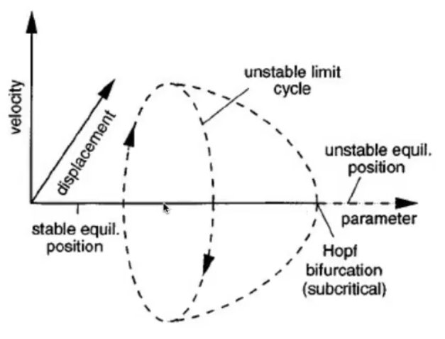
  The bifurcation diagram reports the values visited or approached asymptotically by the system (such as steady states and limit cycles), as a function of the bifurcation parameter $(k)$, thus it is drawn in the plane $(k,x)$.

---

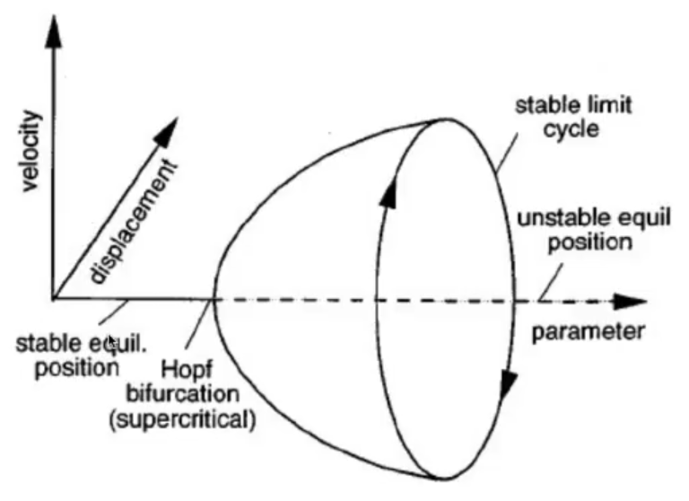
If we analyze the stability of all steady states of a sytem, by changing one of its parameters we will obtain a bifurcation diagram, as we have seen in the supercritical hopf bifurcation and subcritical hopf bifurcation, as we changed the parameter $\beta$.

I recall that the hopf bifurcation is defined as:$\{\begin{array}{l}\dot{x}=\beta x-y+\sigma x(x^2+y^2)\\ \dot{y}=x+\beta y+\sigma x(x^2+y^2)\end{array}$Where $\beta$ and $\sigma$ are parameters and we have that:

• $\sigma =-1$, we will have the SUPERcritical hopf bifurcation.
• $\sigma =+1$, we will have the SUBcritical hopf bifurcation.

Now let’s try to visualize better the meaning behind the bifurcation diagram: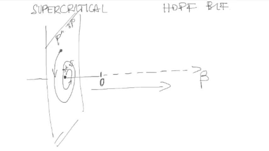

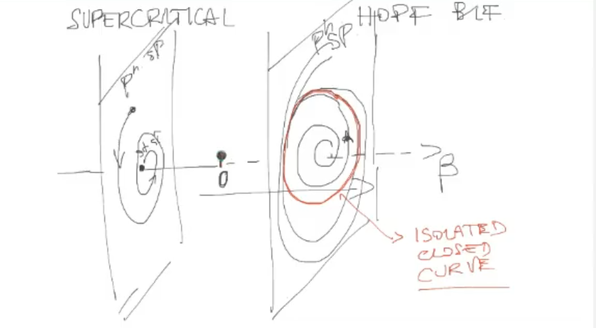
Each point of the bifurcation diagram represents a phase plane/phase space (with infinite inital conditions), and the lines (dotted and continue) represents the stabilities/attracting set of the phase plane: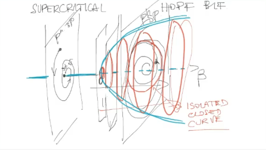

---

Also we have seen the following types of bifurcations:

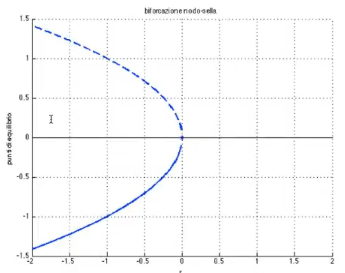
• Saddle-Node bifurcation:
  
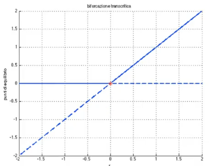
• Transcritical bifurcation:
  
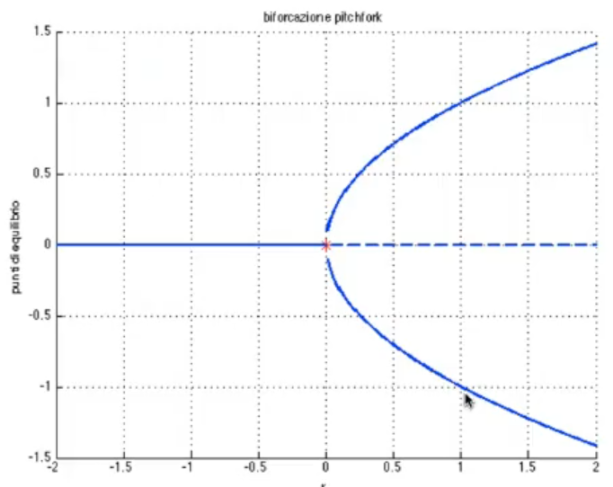
• Supercritical pitchfork bifurcation:
  
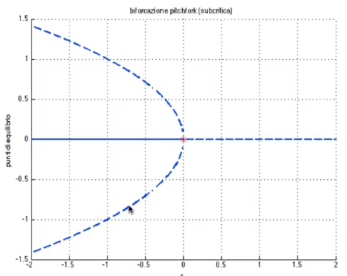
• Subcritical pitchfork bifurcation:
  
• Supercritical Hopf bifurcation (only in continuos time systems):
  
• Subcritical Hopf bifurcation (only in continuos time systems):
  
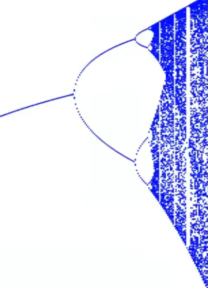
• Flip bifurcation (only in discrete time systems, specifically we have seen it in the logistic equation):
  

---

Let’s see how we can classify them: A bifurcation occurs when there is a drastic change in the flow, in mathematical it means when ==at least one eigenvalue becomes $0$==.

So starting from a point $x_0$ close to a steady state $x^{\ast }$ we can have that:

• The trajectory converges to $x_0$.
• The trajectory converges to a limit cycle.
• The trajectory converges to another point $x_2^{\ast }$.
• The trajectory diverges.

As I will demonstrate with this MATLAB script, and as we have seen thanks to the Hartman-Grobman theorem we can easily find how the stability of the steady states changes after a bifurcation, however we cannot easily find the presence of limit cycles and strange attractors (or any emerging pattern) for those our best bet is to analyze them grafically.

---

Video Lecture References

• Linearization:
• Hyperbolic Steady States:
• Hartman-Grobman Theorem:
• Manifolds: