To solve this exercises you’ll need to use MATLAB. You can make a general script with MATLAB for each of the following points, I didn’t make them, since I’ve had an Oral Exam instead of a Written one, sorry. I just made this kinda general script, but I don’t know if you will find it useful:
For the Dynamic Systems exercises/solutions I have taken as example the Lorenz system. For the Discrete Systems exercises/solutions I have taken as example the logistic equation. Also most of the code you’ll need can be found it in the MATLAB Lab Lectures:
- CDS - Lecture 7
- CDS - Lecture 9
- CDS - Lecture 11
- CDS - Lecture 14
- CDS - Lecture 21
- Follow these lectures and steal their code.
Fax-simile exam/past exams with good explanations and solutions:
Index
- Find the Steady States (Dynamical Systems)
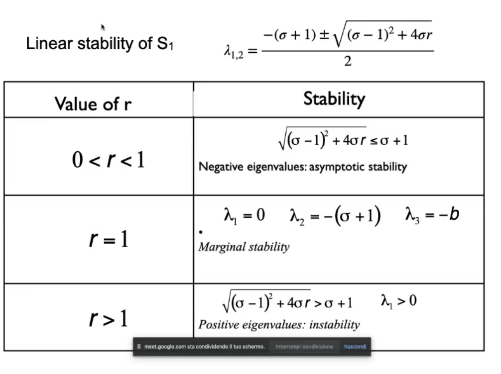
- Study the Stability • Jacobian Matrix (Dynamical Systems)
- Bifurcation Diagrams • Study the Bifurcations (Dynamical Systems)
- Plot the Phase Plane and Phase Space (or Flow)
- Coupled Systems • Graphs • Networks
- Find the Steady States (Discrete Time System)
- Bifurcation (Discrete Time System)
(I DID NOT TEST THESE SCRIPTS, please take them as reference only)
Find the Steady States (Dynamical Systems)
syms x y z k
sigma = 10;
beta = 8/3;
system = [
	sigma*(y-x) == 0
	-x*z + k*x - y == 0
	x*y - beta*z == 0
]
[S_1, S_2, S_3] = solve(system, [x, y, z])
Study the Stability • Jacobian Matrix (Dynamical Systems)
- Find the Steady States (Dynamical Systems)
- Find the Jacobian Matrix:
syms x y z k sigma = 10; beta = 8/3; system = [ sigma*(y-x) == 0 -x*z + k*x - y == 0 x*y - beta*z == 0 ] J = jacobian(system, [x, y, z]) - Find the eigenvalues:
[x y z] = S_1 J_of_S1 = subs(J) eigenvealues_1 = eig(J_of_S1) [x y z] = S_2 J_of_S2 = subs(J) eigenvealues_2 = eig(J_of_S2) [x y z] = S_3 J_of_S3 = subs(J) eigenvealues_3 = eig(J_of_S3) - Plot the real part of the eigenvalues, and calculate where at least one of them is equal to :
This is a little more complex, since you’ll need for eacheigenvealues_iarray, the real part of the 3 eigenvalues inside.
To do this you can use again the ‘subs’ function, the ‘real’ function and finally the ‘plot’ function.
To find if and where at least one of these eigenvalues is/are equal to , I would suggest the ‘solve’ function, similar to before, but you can find the way you prefer to solve this, even graphically if you want. - Study the stability.
Suppose you have plotted the real (and if you want also the imaginary part) of all 9 found eigenvalues, and also found for which at least one eigenvalue is equal to , for the sake of the example suppose you have found and .
For each of these values take a value slighty smaller and onther value slighty larger, like and , substittue them in theeigenvalues_ithat corresepond to them, and see, for :- If the eigenvalues are all negative ⇒ asymptotic stability.
- If at least one eigenvalue is positive ⇒ instability.
- Remeber that you can and should verify this.
- Then do the same for , then also for and for , so that at the end you’ll obtain somenthing like:
Bifurcation Diagrams • Study the Bifurcations (Dynamical Systems)
- Insert the system into MATLAB, similar to this:
function [dot_x, dot_y, dot_z] = lorenz_system(x, y, z, k) sigma = 10; beta = 8/3; dot_x = sigma*(y-x) dot_y = -x*z + k*x - y dot_z = x*y - beta*z end - Find the Steady States (Dynamical Systems)
- Find the Jacobian, and study the stability.
- Plot the Bifurcation Graph.
An example on how to do this is explained in the MATLAB Lab Lecture (14). - Study the Bifurcations: we have seen 6 types of bifurcation for dynamic systems:^study-the-bifurcations
- Saddle-Node bifurcation.
- Characteristics: A saddle-node bifurcation occurs when two fixed points (one stable and one unstable) collide and annihilate each other as a parameter is varied.
- Stability: Before bifurcation, there are two fixed points: one stable and one unstable. After bifurcation, both fixed points disappear, often leading to a sudden change in the system’s behavior.
- Transcritical bifurcation.
- Characteristics: Transient bifurcations are temporary changes in the dynamics of a system due to time-dependent parameters. They are not permanent and revert as the parameter continues to change.
- Stability: The stability changes are transient and revert back once the parameter continues to evolve.
- Supercritical pitchfork bifurcation.
- Characteristics: A supercritical pitchfork bifurcation occurs when a stable fixed point becomes unstable, and two new stable fixed points emerge symmetrically as a parameter passes through a critical value.
- Stability: Before bifurcation, there is a single stable fixed point. After bifurcation, the original fixed point becomes unstable, and two new stable fixed points appear.
- Subcritical pitchfork bifurcation.
- Characteristics: A subcritical pitchfork bifurcation occurs when a stable fixed point becomes unstable, and two unstable fixed points emerge symmetrically. As the parameter passes through a critical value, the system can exhibit a jump to one of the new stable branches.
- Stability: Before bifurcation, the fixed point is stable. After bifurcation, the original fixed point becomes unstable, and two unstable fixed points appear.
- Supercritical Hopf bifurcation.
- Characteristics: A supercritical Hopf bifurcation occurs when a fixed point becomes unstable, and a stable limit cycle (oscillatory behavior) emerges as a parameter passes through a critical value.
- Stability: Before bifurcation, the fixed point is stable. After bifurcation, the fixed point is unstable, and the system exhibits stable oscillations.
- Subcritical Hopf bifurcation.
- Characteristics: A subcritical Hopf bifurcation occurs when an unstable limit cycle exists for parameter values below the critical value. As the parameter passes through the critical value, the limit cycle disappears and the fixed point becomes unstable.
- Stability: Before bifurcation, the fixed point is unstable. After bifurcation, the fixed point remains unstable, and there may be a sudden appearance or disappearance of an unstable limit cycle.
- Saddle-Node bifurcation.
- ~Example:
Looking a this INCOMPLETE graph: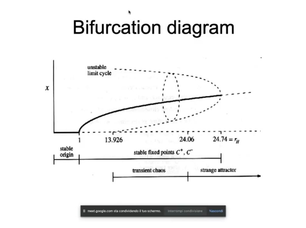
It is INCOMPLETE since there is another unstable limit cycle mirrored with respect to the abscissa, that is not reported here.
You need to identify the bifurcations like so: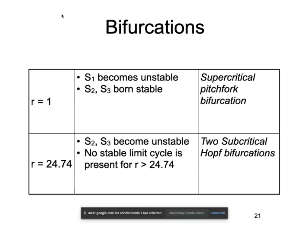
Plot the Phase Plane and Phase Space (or Flow)
- Define the system.
- Take random initial condition: .
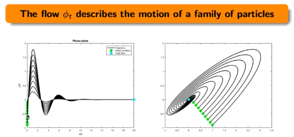
- For the dynamics graph how each variable of the system (~ex.: ) evolves by incrementing from to an arbitrary number , and plot all the variable in the same 2D graph.
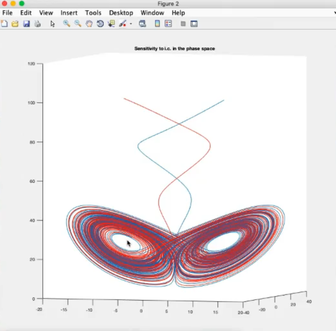
- For the phase space plot in a 3D space (it depends on how many variables you have, in this case we have 3 variables so a 3D space) how the system evolves for to , like before by incrementing from to an arbitrary number .
- Here’s an example in 2D of both dynamics and phase plane/phase space:
- Here’s an example in 3D of the phase space of the Lorenz system in the chaotic regime:
Coupled Systems • Graphs • Networks
- Define the systems (at least systems are necessary), for example let’s take the 1st exercise of the 2015_12_21 exam:
- In these systems you to have a parameter (~ex.: ) that “binds” two variables of the two systems, like:
- (Optional) Draw the graph, and define the matrix:
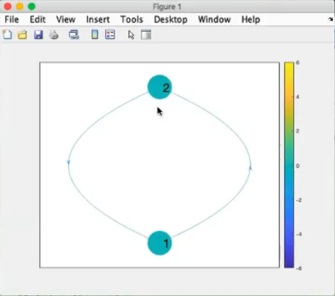
And the Matrix will be:This matrix means that the node 1 (representing the first system) is connected to node 2 (the second sysmtem), since we have the term: in the first sysmtem.
And also that the node 2 is also connected to node 1, since we have the term in the second system.
For reference: - Plot the evoulution of the two system for diffrent values of , the plot can be done component-wise or system/node-wise, somenthing like:
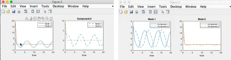
This plot are basically plots of the dynamics.
- A “strange/difficult question”: “Report a brief description of the two systems”
- Fax-Simile Answer: “The first systems is the Rossler system, the second system is the normal form of the Hopf bifurcation”. (from the 2015_12_21 exam)
- NOTE: we have seen many system that you need to memorize:
- A “strange/difficult question”: “Can you summarize all the results in a single sentence?”
- Fax-Simile Answer: “The coupling stabilizes the two systems and eliminates oscillations”. (from the 2015_12_21 exam)
- A “strange/difficult question”: “Discuss the obtained results by comparing them with the solutions of the uncoupled sysmtem?”
- Fax-Simile Answer: “Stable steady states are stronger than oscillations.
Period-1 oscillations are stronger than period-2nT (period-2, period-4, period-8, …) oscillations and chaotic oscillations”. (from the 2015_12_21 exam)
- Fax-Simile Answer: “Stable steady states are stronger than oscillations.
Find the Steady States (Discrete Time System)
- Given the system:Like for example:
The steady state are values such that: - So for the logistic equation, since it is a second order equation, we will find 2 steady states:
- You can automatically find the steady states in MATALB, similar to how we found them for the dynamical case.
Bifurcation (Discrete Time System)
The steps are similar to the bifurcation in dynamical systems, but there are some differences.
- Find the Steady States (Discrete Time System)
- Find the derivative of the discrete function
- Study the stability for each found:
- If : then the steady state is asymptotically stable.
- If : then the steady state is unstable.
- If : then we cannot say anything about the stability of .
- Plot the bifurcation diagram, in MATLAB it will be much simpler than for the dynamical case.
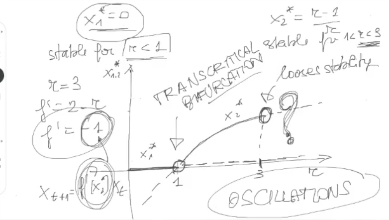
- Using the study of the stability and the bifurcation plot, study the bifurcations:
- saddle-node bifurcation, transcitical bifuracitions, supercritical/subcritical pitchfork bifurcations are the same as for the dynamical case.
- For the discrete case however, we have that there are no supercritical/subcritical Hopf bifurcations, but there can be flip bifuractions.
- Flip Bifucration: If the derivative evaluated in the steady state is equal to for some values of the parameter :This definition is given in the 2nd execrise of the 2015-09-17 exam.
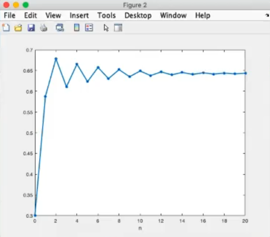
- Flip Bifurcation: we have seen that a flip bifucation occurs for the logistic equation for , when the steady states loose stability and “undumped oscillations” begin to occur after this value:
Let’s see some examples to better understand the “flip bifurcation”:- For ():
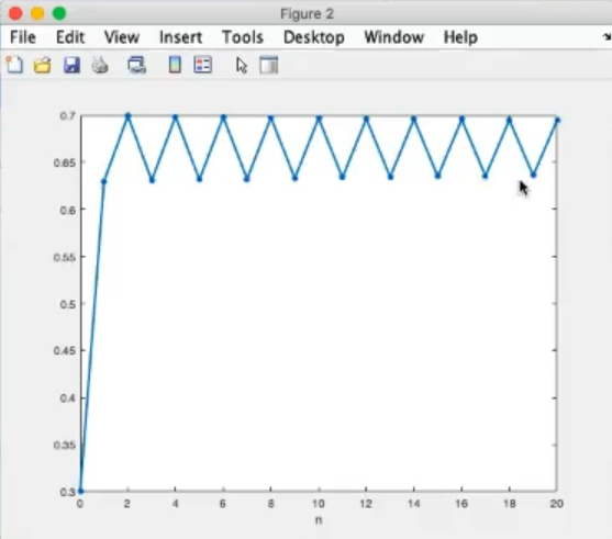
- For :
- For ():
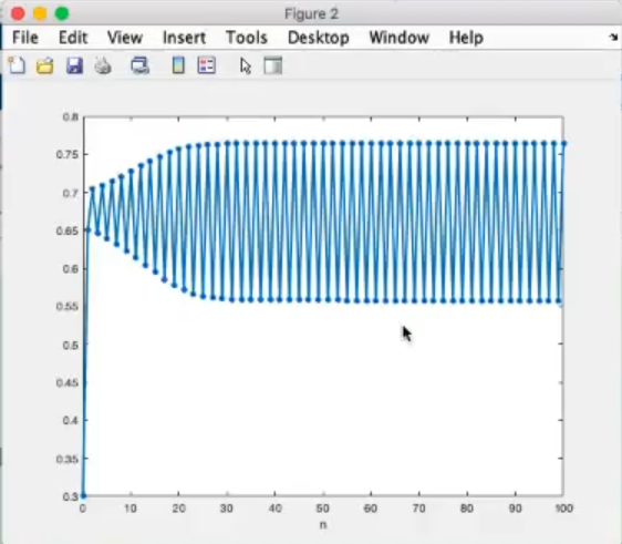
- For ():