CDS - Lecture 4

---

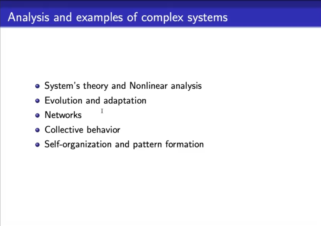
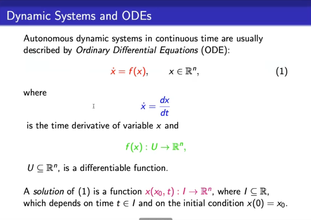
• We are not interested/we don’t care about solving for $x(t)$ analytically, we will not find the formula, at most we will solve it numerically, that means, solving using numerical data, giving $x(t)$ and $t$ actual values.

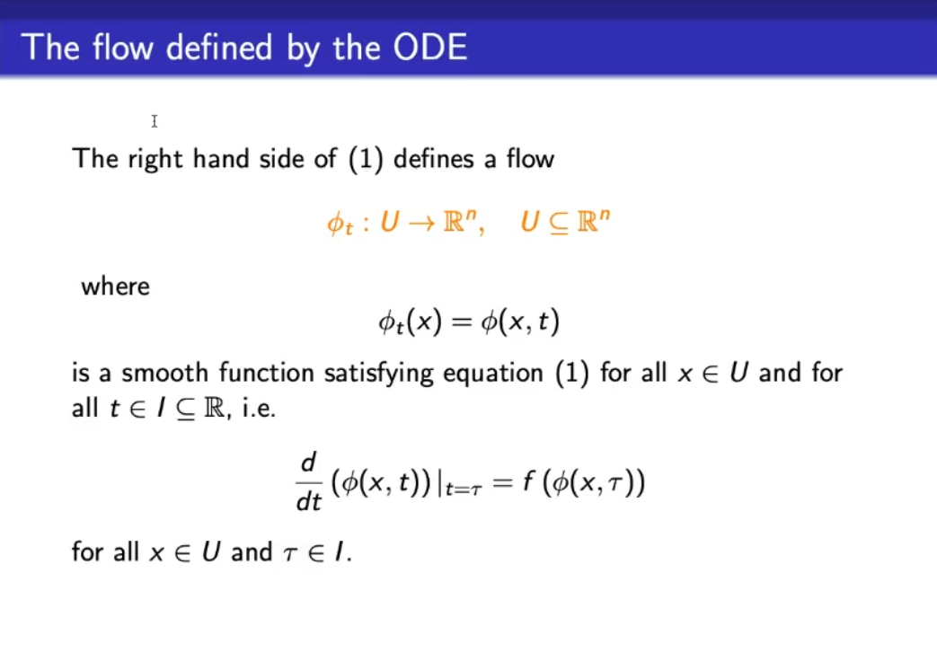
• Consider the flow as an “image” of the function $\dot{x}=f(x)$ for some $t=\tau$ and initial state $x_0$, where: $x_0=x(t={\tau }_0)$.

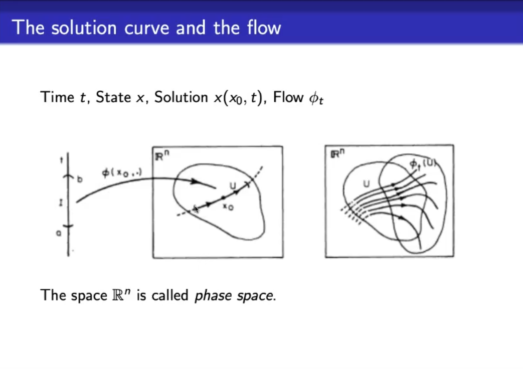
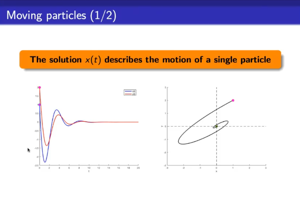
• In first picture we use a single initial condition, in the second we use many initial conditions, to see how the system evolves.

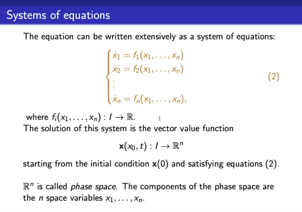
• $x$, so $x_0$ as well, are vectors, while $t$ the time is a scalar, so $t\in \mathbb{R}$.

• Here’s the example in which $x\in {\mathbb{R}}^2$
• In the first graph we represent $x_1(t)$ and $x_2(t)$
  • $x_1(t)$ is called $x(t)$
  • $x_2(t)$ is called $y(t)$
• In the second graph we represnt the flow, however it misses the arrows that indicate the flowing of time.
• If we were to take $x\in {\mathbb{R}}^3$ we would need a 3D graph to represent flow.
• The first graph is called dyncamics graph, the second phase space.

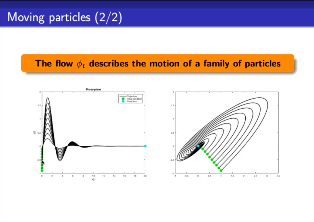
• If we take many different initial conditions

• So when desining the geometry of the phase space, then we will have that a solution in the phase space CANNOT intersect itself, still under the hypotesis that $f$ is a differentiable function.

• eigenvectors ??? and eigenvalues ???TODO

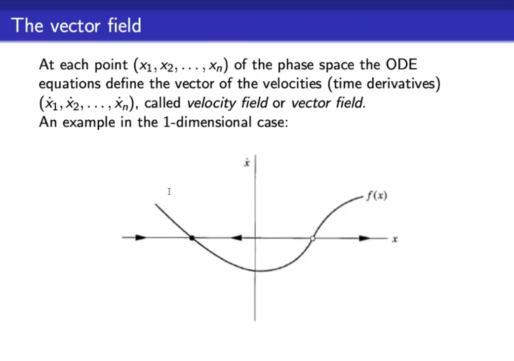
• This is an example of how we can study the geometry of the steady state.
• The black point is a STABLE steady state, also called “attractor”.
• The white point is a UNSTABLE steady state*.
• The arrows define how ???TODO the system evolves / the initial condition evolves
• $\dot{x}$ can also be seen as representig the velocity, as you can see the velocity decreases as you approach the stady state.

• IMPORTANT
• In case of linear system we need the nullclines, and eigenvectors, to define the phase space.

---

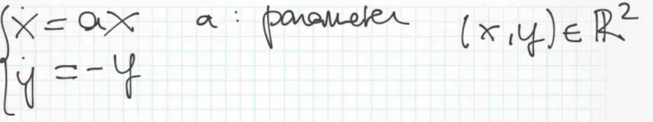
• This is a special linear system, $\dot{x}$ depends only on $x$ and $\dot{y}$ depends only on $y$.

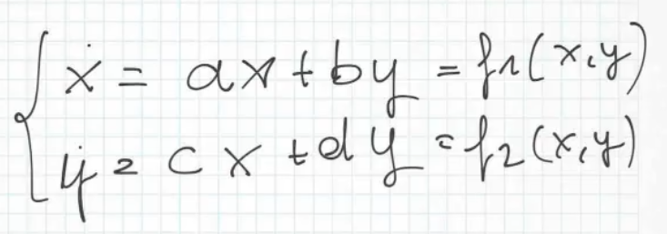
• General case.

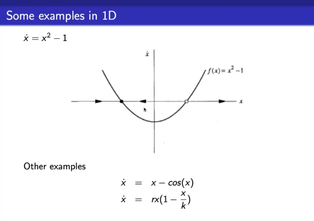
If we solve analytically we find:$x(t)=c{e}^{at}$We can define:$x_0=c{e}^{a\cdot 0}=c$And we can find:$\begin{array}{l}x(t)=x_0{e}^{at}\\ y(t)=y_0{e}^{-t}\end{array}$However remeber, that we will not find analytic solutions.

We can represent the graph 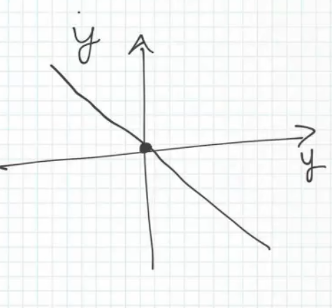$\dot{y}=-y$:

• $y=0$ is a steady state.

Let’s represent the flow:
On the right of the ss (steady state) the derivitave over time ($y$) is positive.
While on the left $\do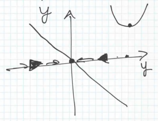t{y}<0$, so:

• As we can see $y=0$ is a stable steady state.

Now we can study $\dot{x}=ax$, notice that $a$ can assume different values, mainly we will focus on $a>0$ and for $a<0$. For $a<-1$, basically the graph is the same as before (for 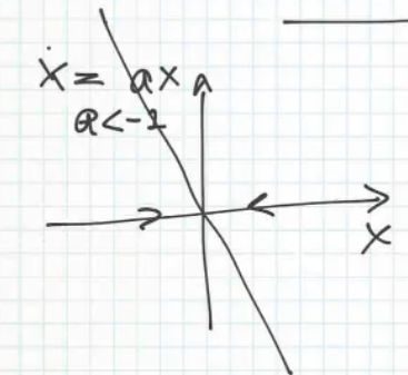$\dot{y}=y$):

Let’s combine this two solutions, and let’s draw the nullclines, so let’s find for $\dot{x}=0$ and $\dot{y}=0$, so:$\begin{array}{l}\dot{x}=0\Rightarrow x=0\\ \dot{y}=0\Rightarrow y=0\end{array}$For this case preatty simple, let’s draw the nullclines: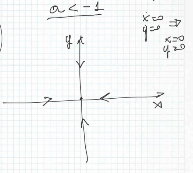

Now we can represent the flow: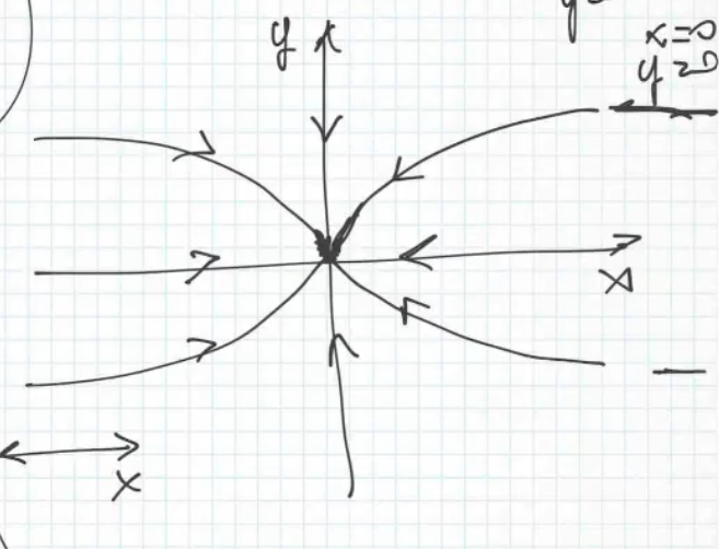

• For $x\to \infty$ we have that the flow will be parallel to the $x$ axis.
• For $x\to 0$ (the ss) we have that the flow will be parallel to the $y$ axis.

If we represent the “motion of a family of particles” (the flow 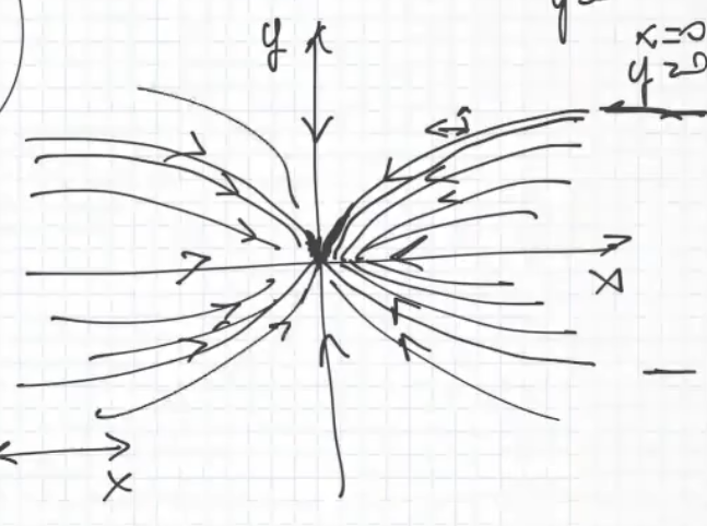${\varphi }_t$):

• This form is becasue $a<-1$, so the velocity along $x$ is higher than the velocity along $y$.
• The velocities we said can be seen as $\dot{x}$ and $\dot{y}$.

If we take 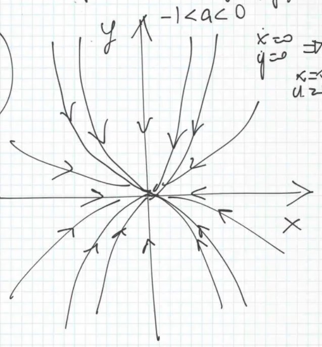$-1<a<0$:

Special case for 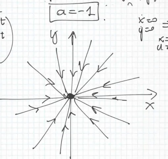$a=-1$:

• In all of these cases the node is called “node”.
• In this particular case, it is called a “node star”

Let’s see what happens for 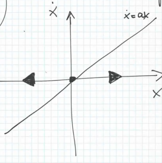$a>0$:

• This is an unstable steady state, since:
  • $\dot{x}\to 0^{+}>0$
  • $\dot{x}\to 0^{-}<0$

The nullclines changes: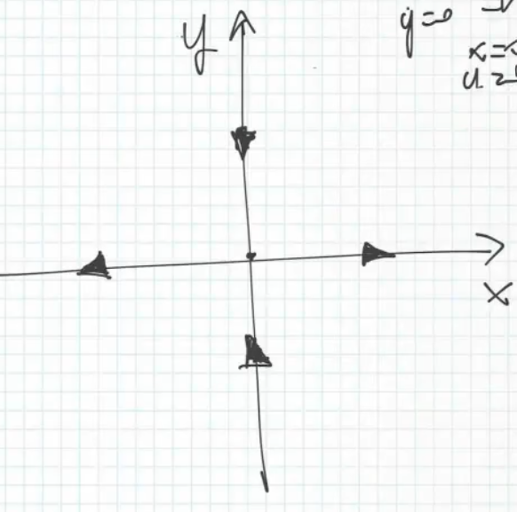

If we represent 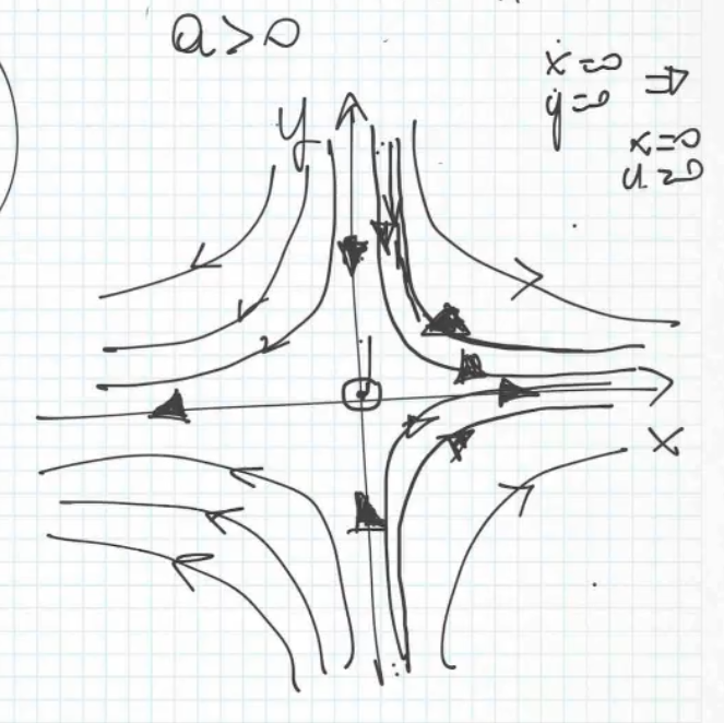${\varphi }_t$ :

• All initial condition will diverge, except and initial condition such that it lies along the $y$ axis, so for $x=0$.
  • For $x_0=0$ the system will converge to $0$.
  • For $x_0\ne 0$ the system will diverge.
• So one component converges $(y)$ and another $(x)$ diverges, for this reason this graph is called a “saddle”, sincenot-sure-about-this

For 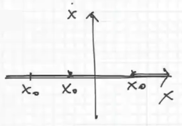$a=0$:

• We cannot represent any arrow, and it said to be marginally stable.

And the flow 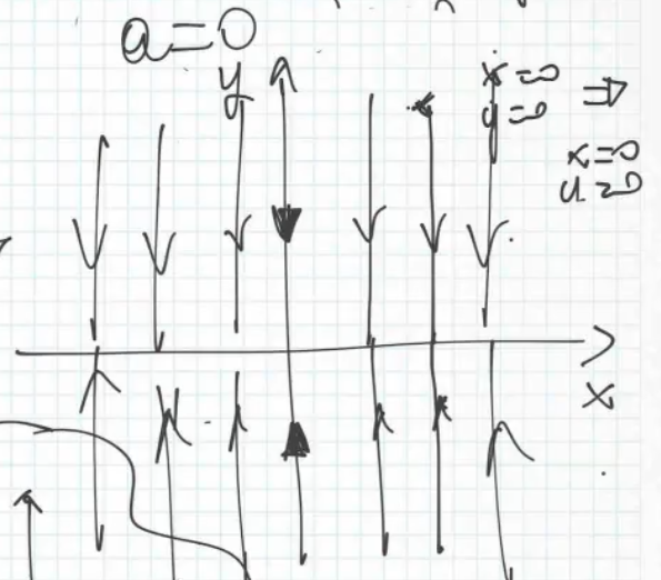${\varphi }_t$ for $a=0$:

• Called “line of steady states”.

As a sneak-peak for the future, in this system we can define the eigenvalues as: ${\lambda }_1=a$ and ${\lambda }_1=-1$, the sign of the eigenvalues is strictly correleted to the stability of the steady states.

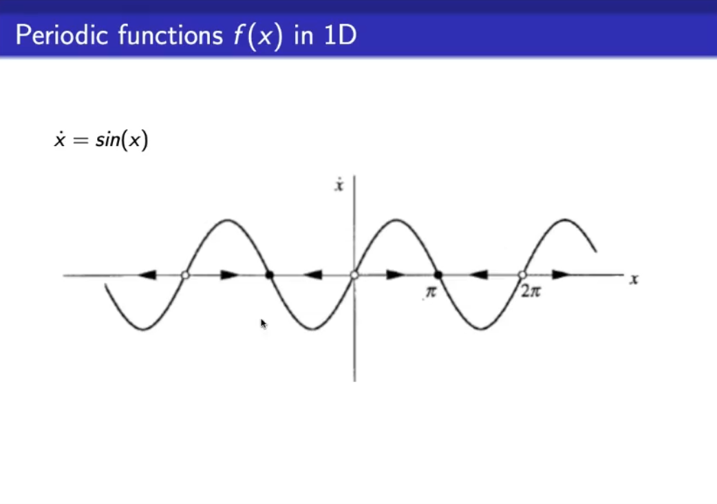
• This function is periodic over $x$, however monodimensional system cannot present periodicity over $t$, nor oscillations.
• As a sneak-peak: we’ll need imaginary eigenvalues in a multidimensional system to have oscillations.

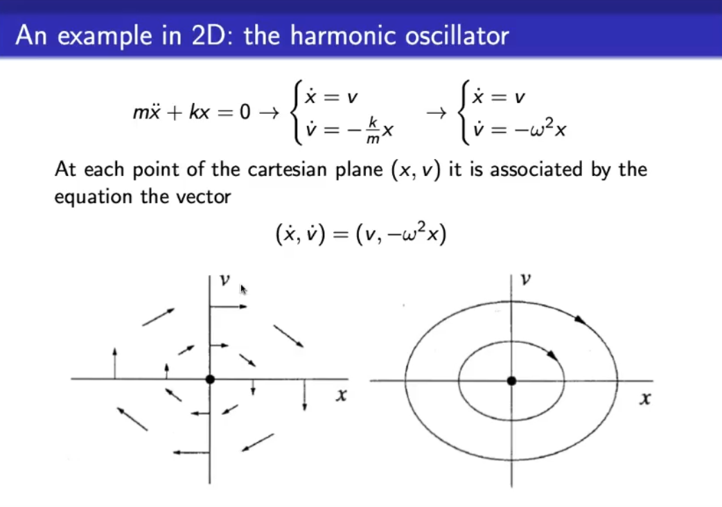
• mass-spring system (no damper).
• Since $\dot{x}\propto v$ (or because $\dot{v}\propto x$) we can call this system “coupled”.