CDS - Lecture 18

These metronomes started with different initial conditions, will syncronize, due how the “system is built”.
Generally we can say that to create a syncronization between multimple systems, we need to create a connection between them, in this example the connection is the plank suspended on two cans of soda.
Syncronization happens in particular networks.
Syncronization is one of the simpler example of “self-organization”.

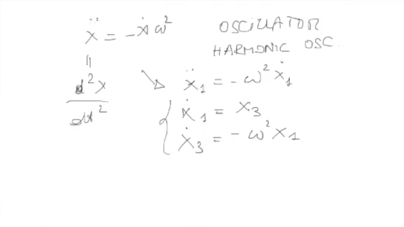
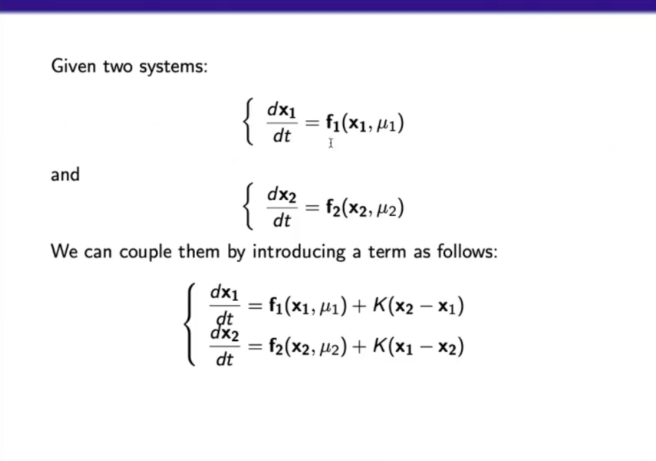
Simple harmonic oscillator

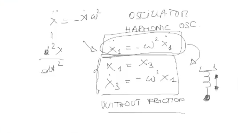
Represents for example a mass-spring system without friction.

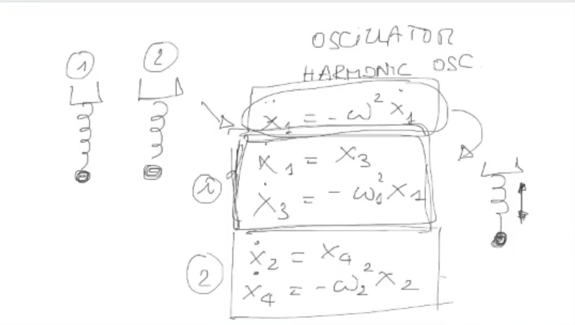
Consider annother equivalent system (it will have different initial conditions, but same differential equations)

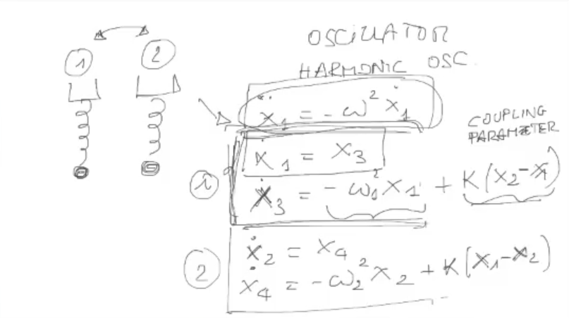
Leaving the first equaiton untuched (since it serves only to define $\overset{x}{¨}$ in terms of ODE equations), we can add a term called “coupling parameter” that depends on a variable of the second system.
I rewrite here the equations: ${x_{1} = x_{3} x_{3} = - ω_{1}^{2} x_{1} + k (x_{2} - x_{1}) {x_{2} = x_{4} x_{4} = - ω_{2}^{2} x_{2} + k (x_{1} - x_{2})$
NOTE: for $x_{2} = x_{1}$ this term is equal to $0$ ⇒ This term is active only when these two variables are different.

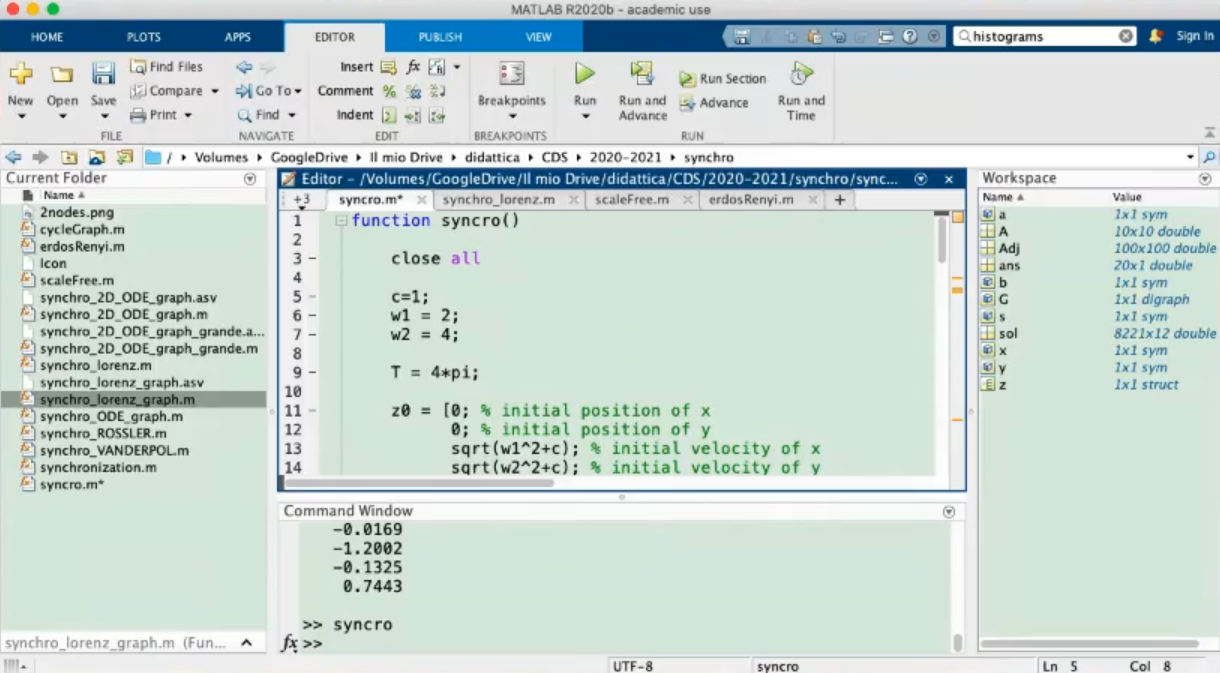
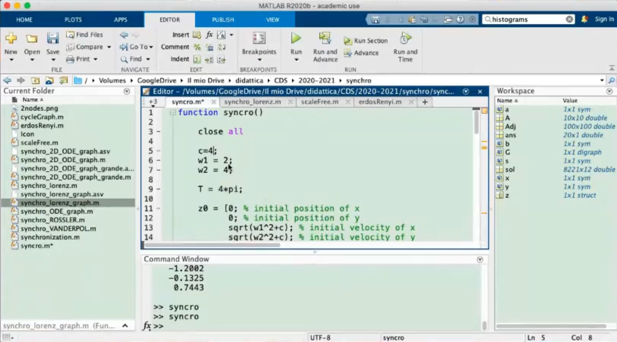
$c$ is the coupling term, previosly called $k$ .

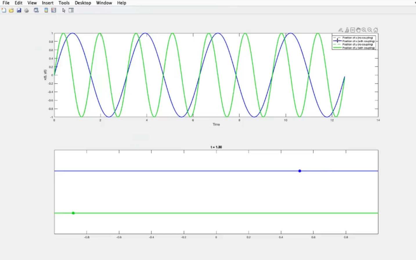
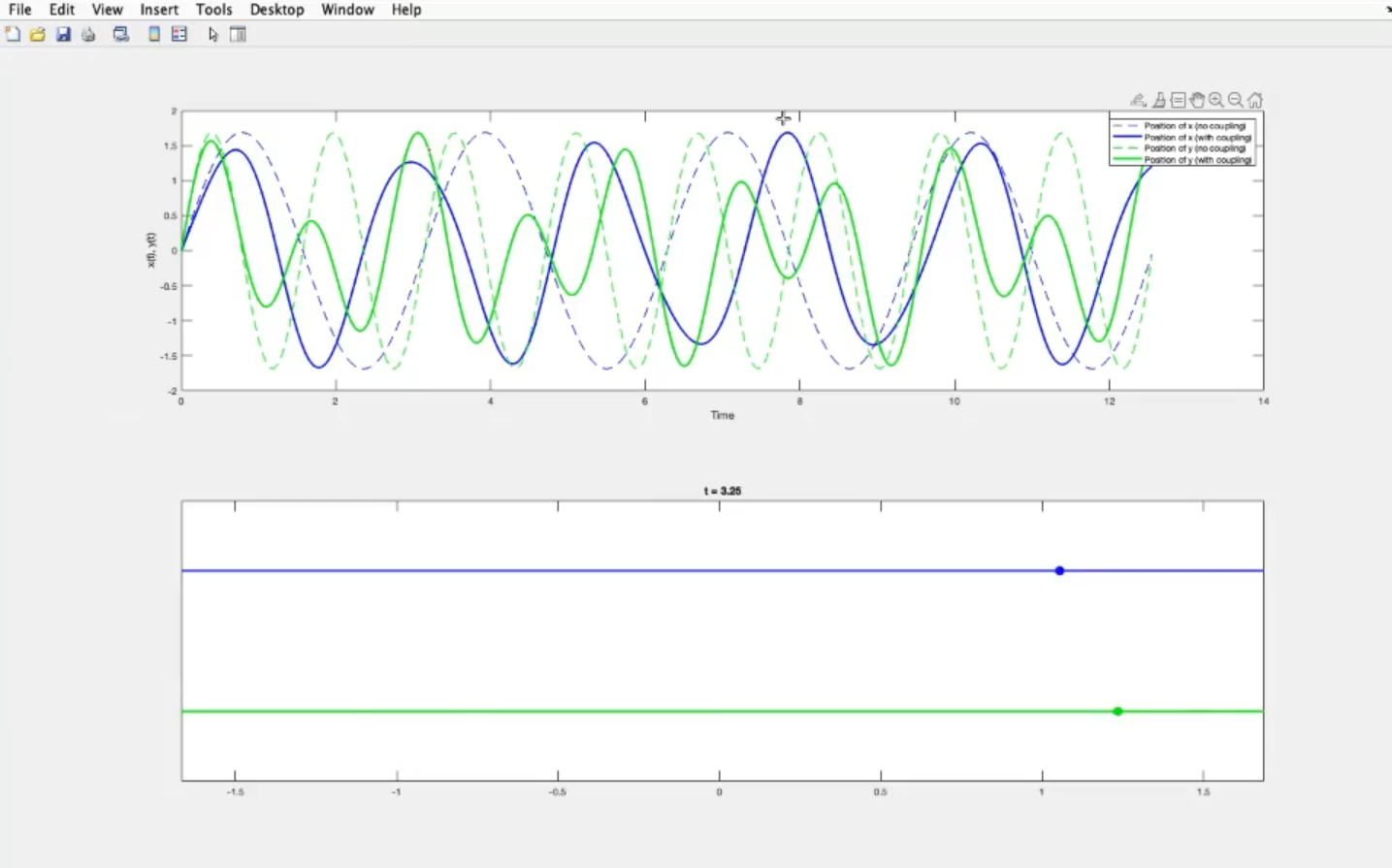
Positions of the two systems.
This graphs are without coupling, $c = 0$ .

$c = 1$ , now there is coupling.

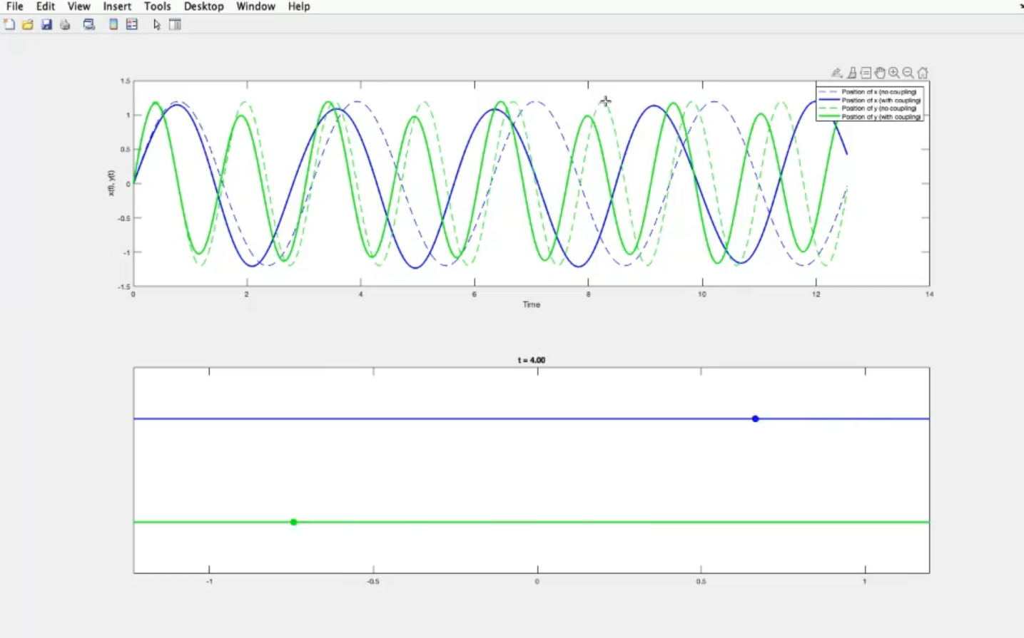
The continous lines are the real systems (with coupling), the dotted line are are the systems without coupling (seen before).

$c = 4$ .

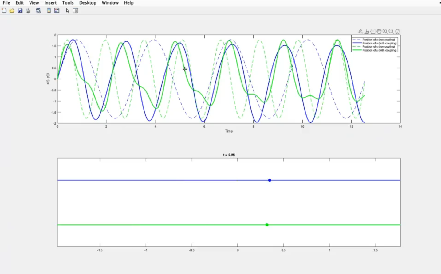
$c = 10$ , we can see that the two lines are much more similar.

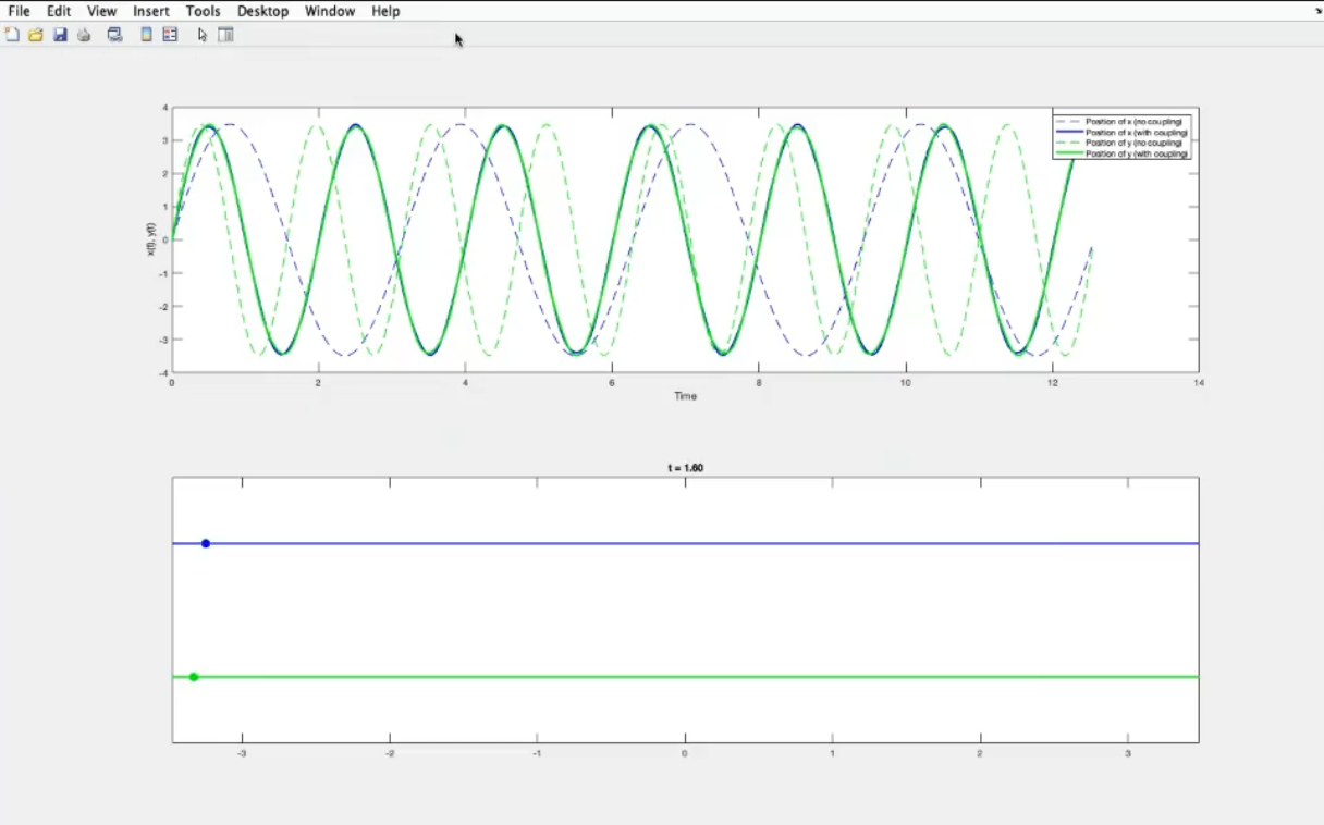
$c = 100$ , almost perfect marching.

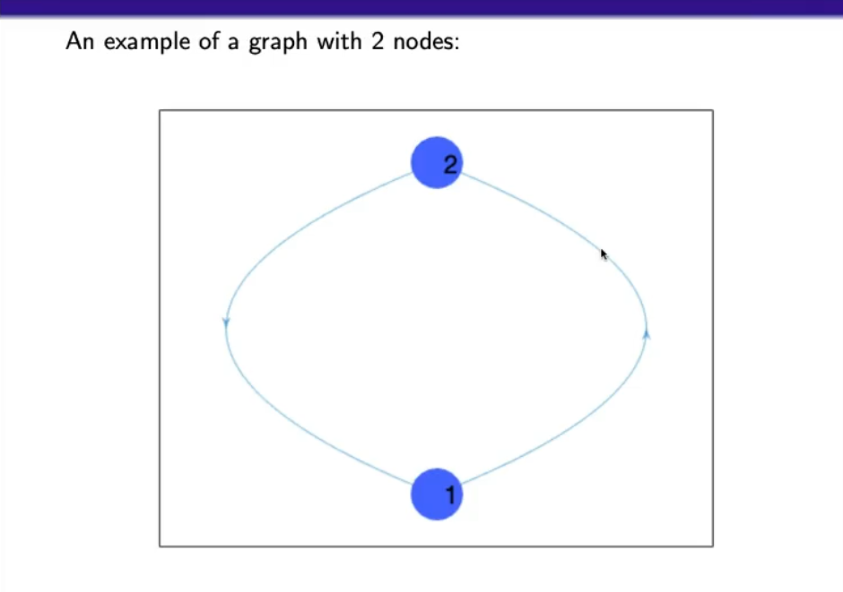
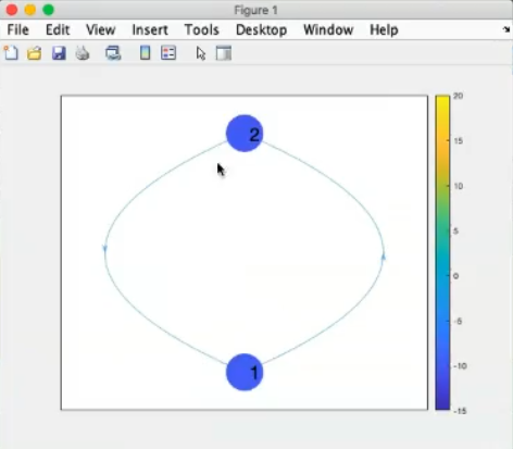
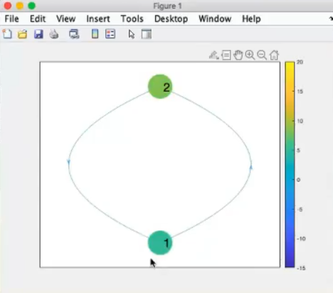
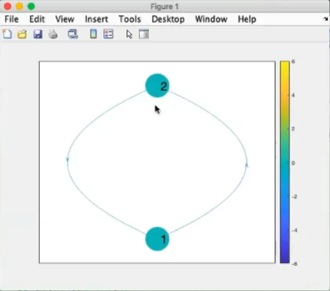
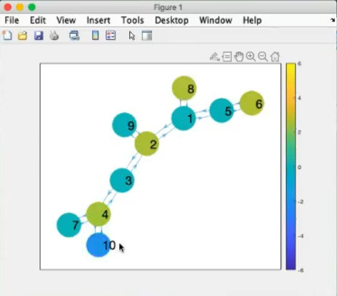
Graphical representation of the connection.
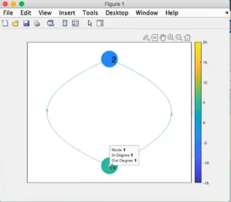
Each node is a system.
REMEMBER: A graph is a mathematical object defined by a given number of nodes and a given number of links connecting the nodes
A graph has many properties, it can be directed or undirected, in this case the graph is directed, since there is a “direction of influence” (the links have arrows).
We will se also other properties.

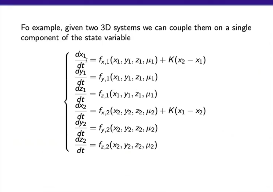
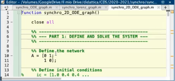
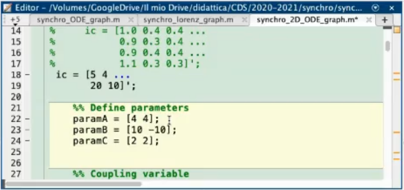
Now immagine that the simple 2-node graph seen previusly describes two Lorenz systems, connected.
Also consider a “weak coupling”, such that only the variable $x_{1}$ of the two system is connected to each other: $k (x_{1}^{'} - x_{1}^{''})$ and $k (x_{1}^{''} - x_{1}^{'})$ .
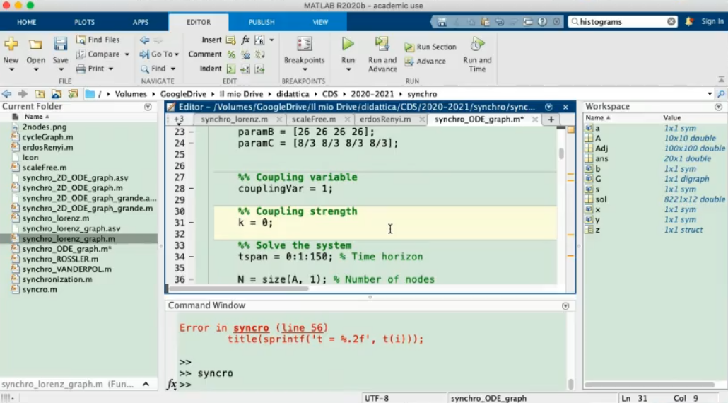
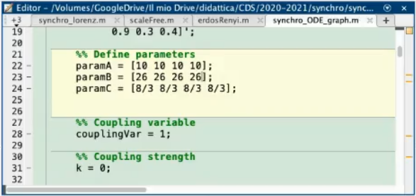
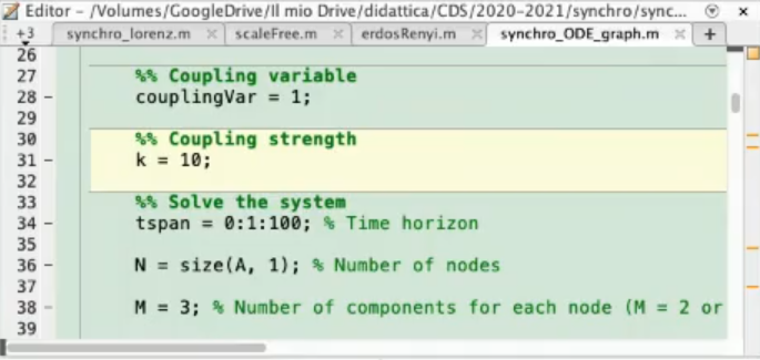
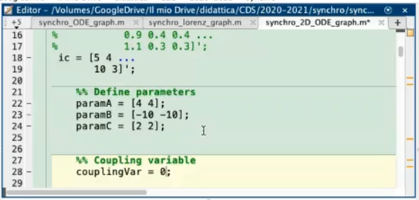
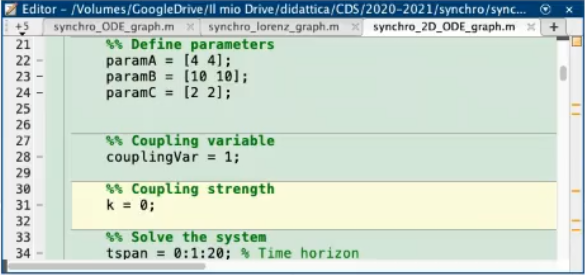
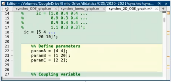
Base example with $k = 0$ (so we are in the case of no-connection / independent systems), and these are the intial conditions and parameters of the two systems:
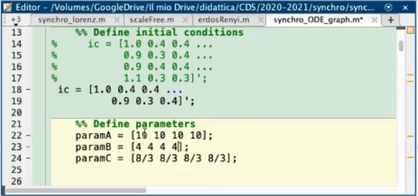
- paramB: isTODO
- paramC: isTODO should be $σ$ or somenthing.

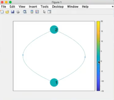
The color represents the value, it does not change much and it remains near $0$ .
It is more or less stable.

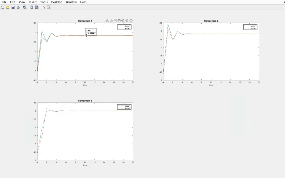
After solving the system, this are the results, since the system is stable, both system convergee to the same results.
We hare in the case of “after the pitchfork bifurcation”TODO LINKS TO LORENTS SYSTEM.

Here we see the same graphs as before, but divided into the two systems, as you can see the only difference is the transients.
REMEMBER: We are in the case of indipendent systmes, they converge to the same results because they have the same parameters and are “converging systems”.

We now move the system into the chaotic regime, by changing paramB.
Still $k = 0$ ⇒ indipendent systems.

The node now change colors frequently, and can assume different colors at the same time, here’s another shot:

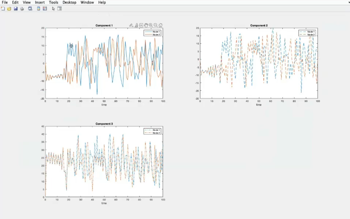
Division in components, you can see the chaos.

$k = 1$ , results are almosts the same as before.

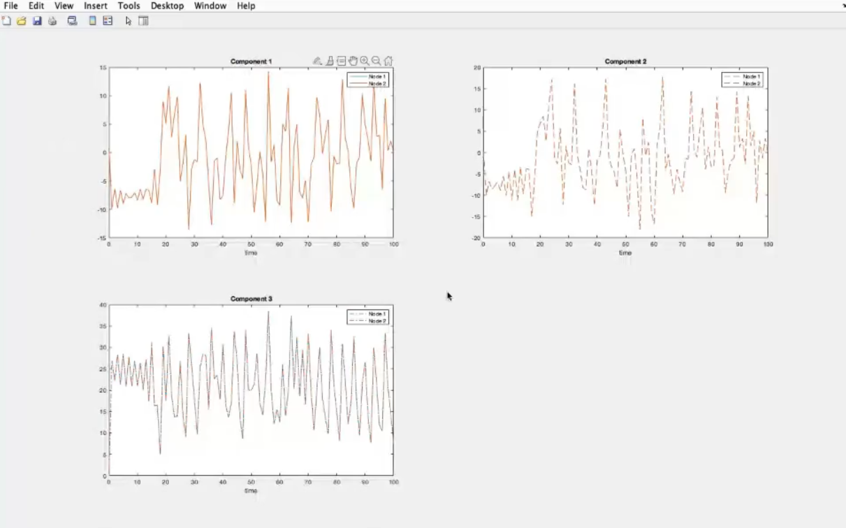
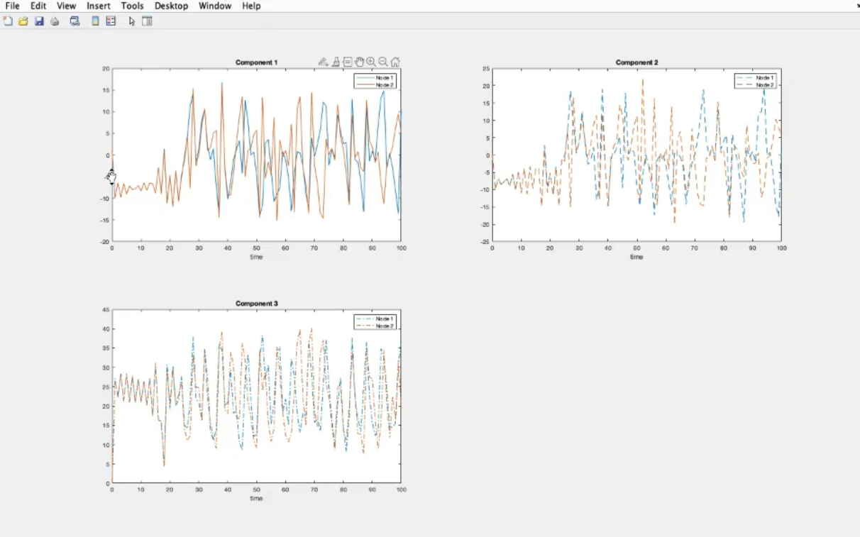
$k = 10$ , much more similar systems ⇒ the two systems are syncronized.
So we have seen that chaotic system can syncronize.

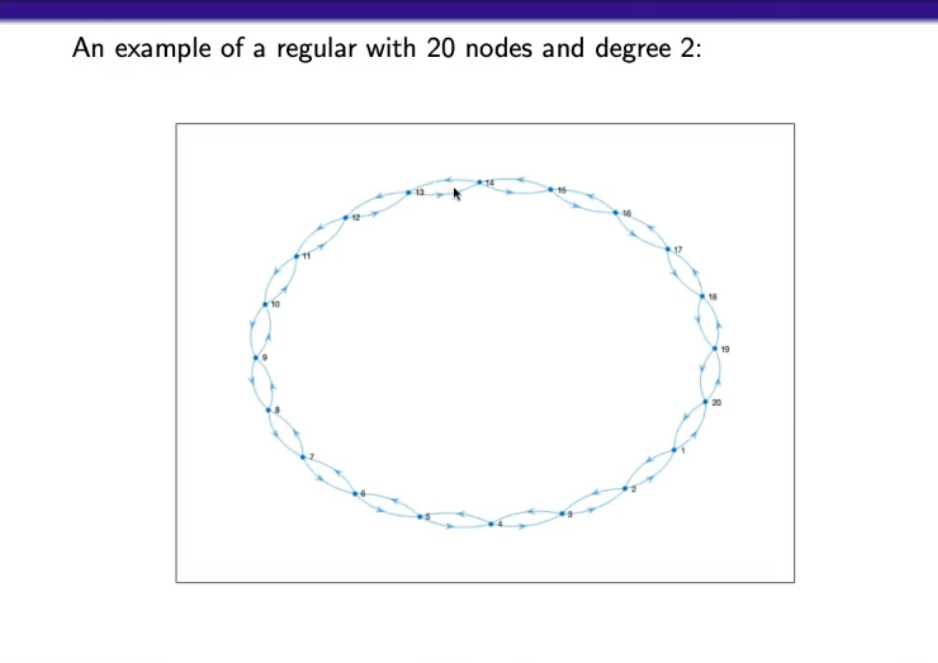
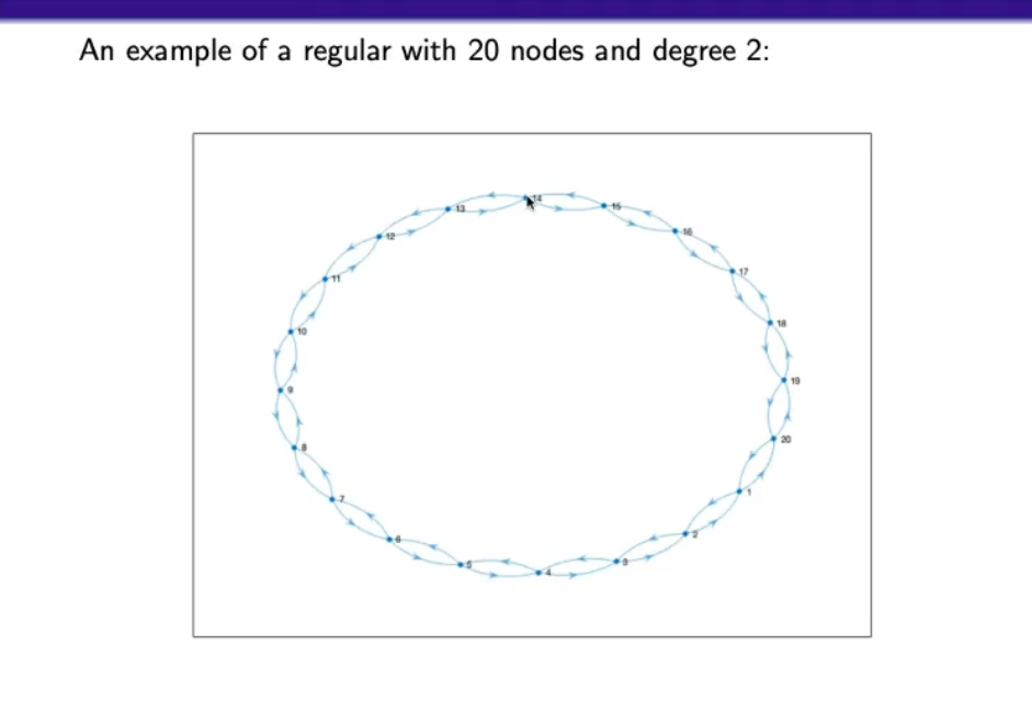
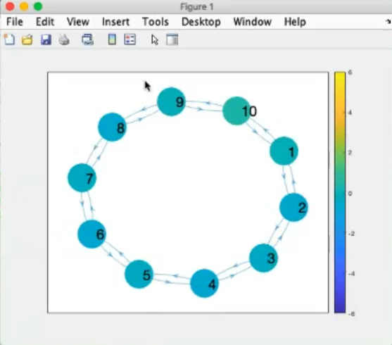
Bidirectional connections.
This is called a “ring network”.

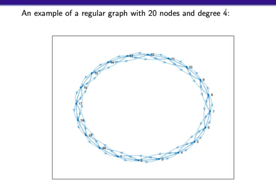
degree 4: each node is connected to 4 nodes.

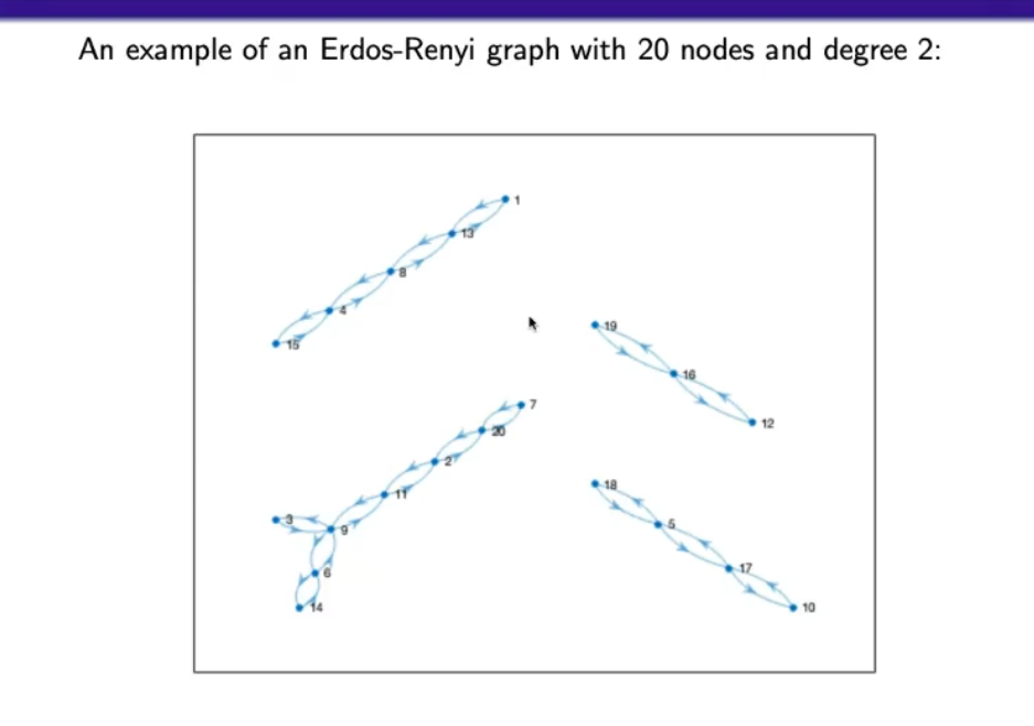
Erdos-Renyi: random graph, in this case degree 2 refers to a medium of connections.

The 12° node is called a “leaf” (it has very few connections)

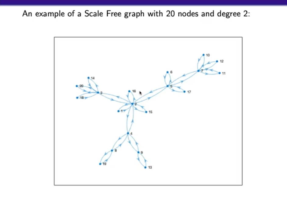
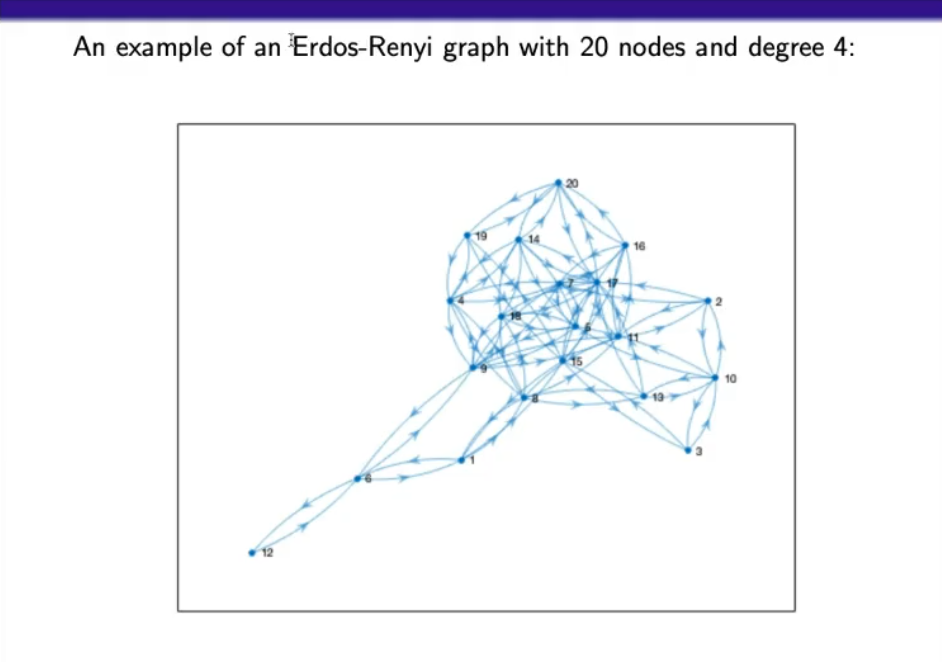
There is only 1 graph (we can always find a list of connections from one node to another)
We can define some hubs like node 2, 3, 4, 5, 7.

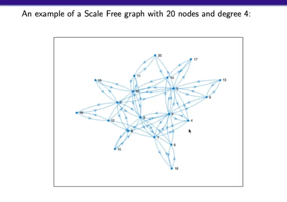
Still some hubs and leaves.

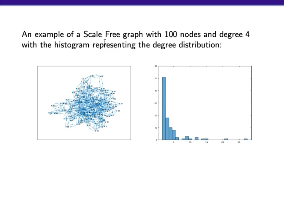
Many leaves (nodes with little connections).
Few higher degree nodes, from the picture we can define the hubs.

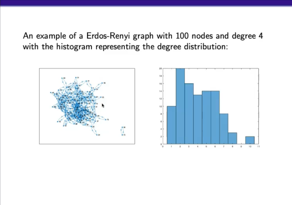
There can be separation (not all nodes can reach all the others)
The maximum degree is lower thatn that of the “Scale Free graph”.

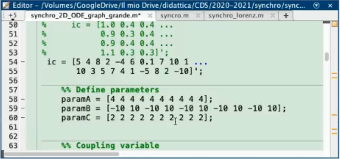
Each node represents a dynamical system.
We will see how different type of graph handle changes, how the change of a node can spread, and the syncronization.

Simplest graph with only 2 nodes.

2 Identical stable systems, with different inital conditions, and NO coupling.

Graph

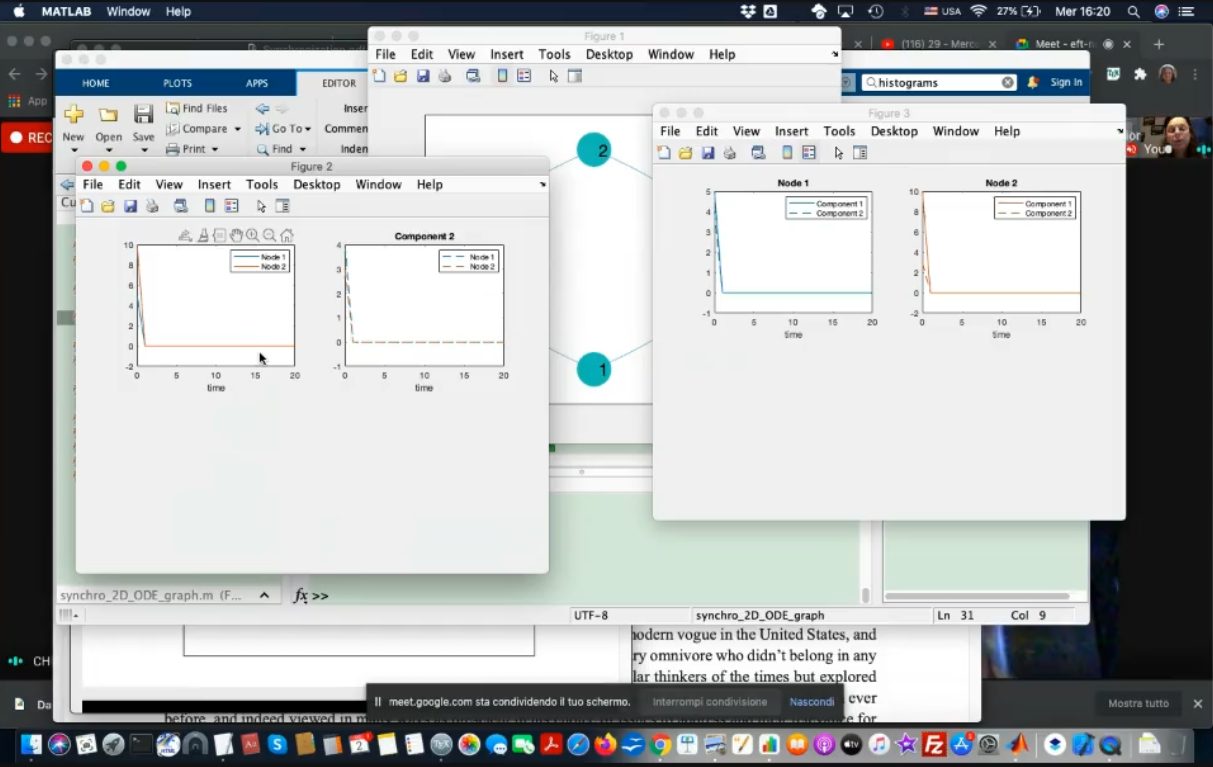
Changing paramB, the systems will now oscillate.

The two system are slightly different, due to the different inital conditions

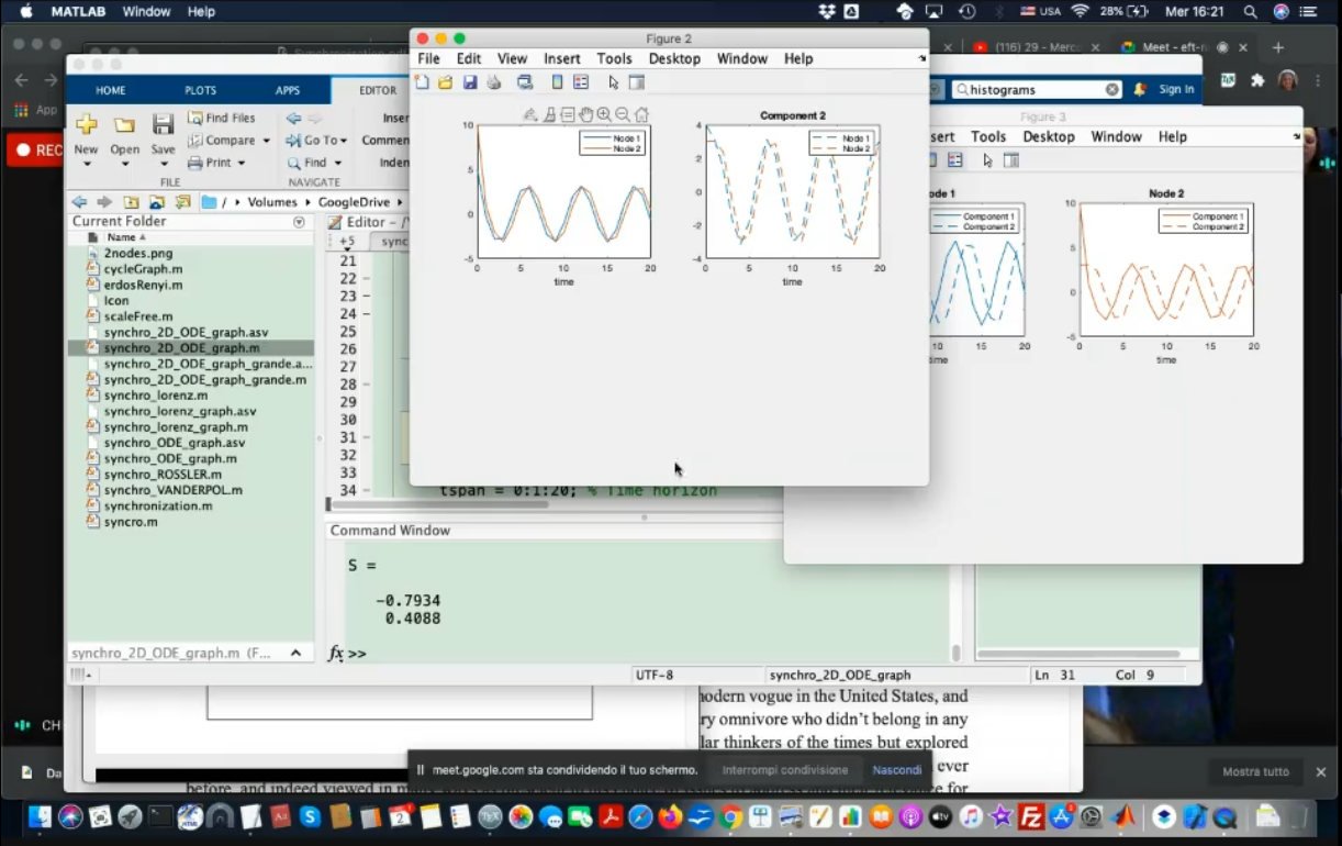
Changing paramB, this time the systems are diffrent.

One oscillating and one converging system

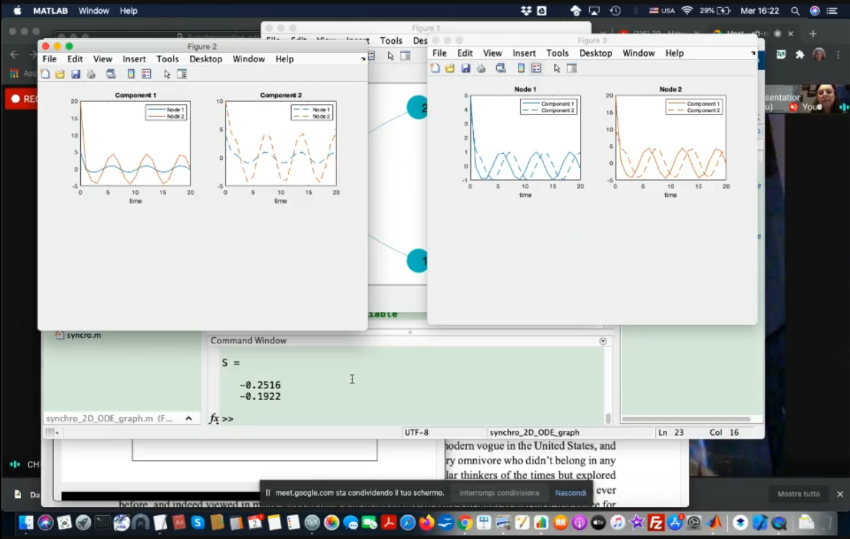
We now introduce coupling: $k = 1$ . (pretty weak)

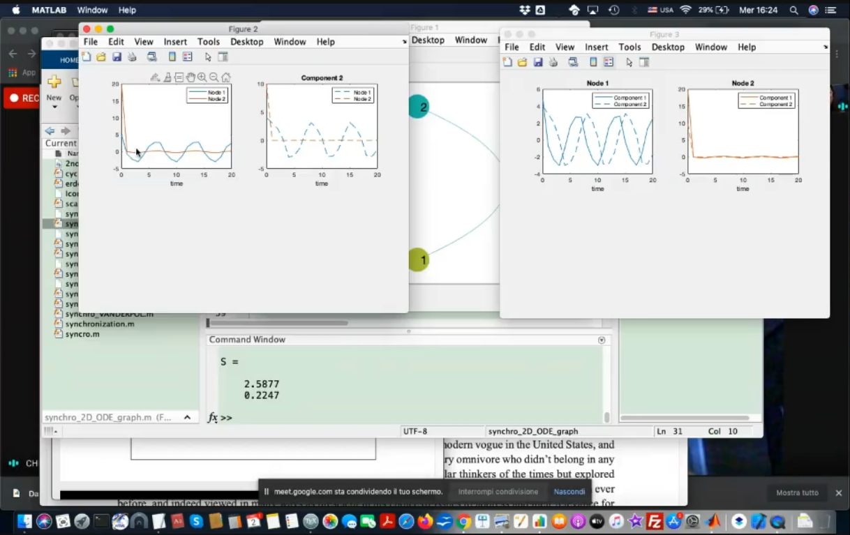
We can see some effects, but since $k$ is small, not very much.

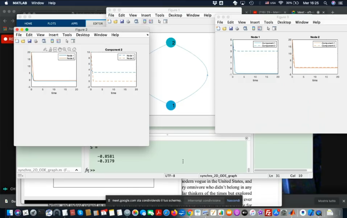
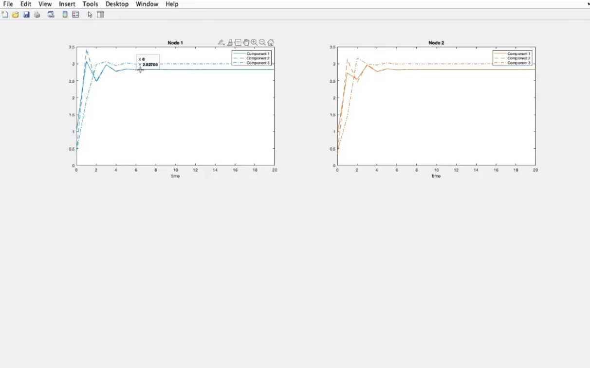
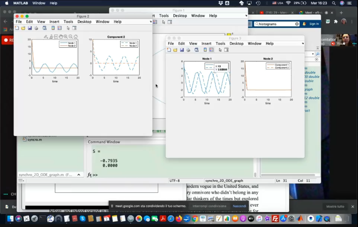
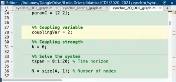
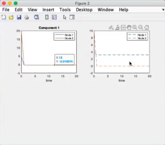
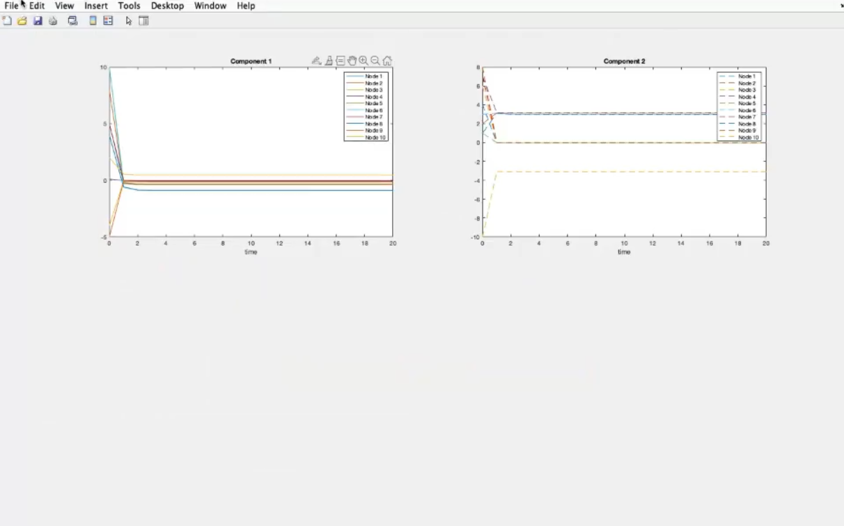
$k = 6$
Now both system converge, however the 2nd components converge to different values, specifically to $- 1$ and the other to $3$ .
The 1st component of both systems converge almost to the same value, since these are the coupled components.

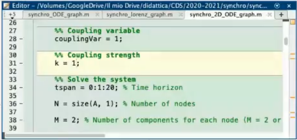
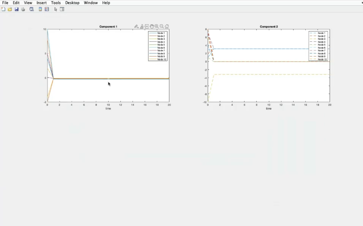
We switch coplingVar from 1 >> 2, meaning that now the coupled components are the 2nd ones.

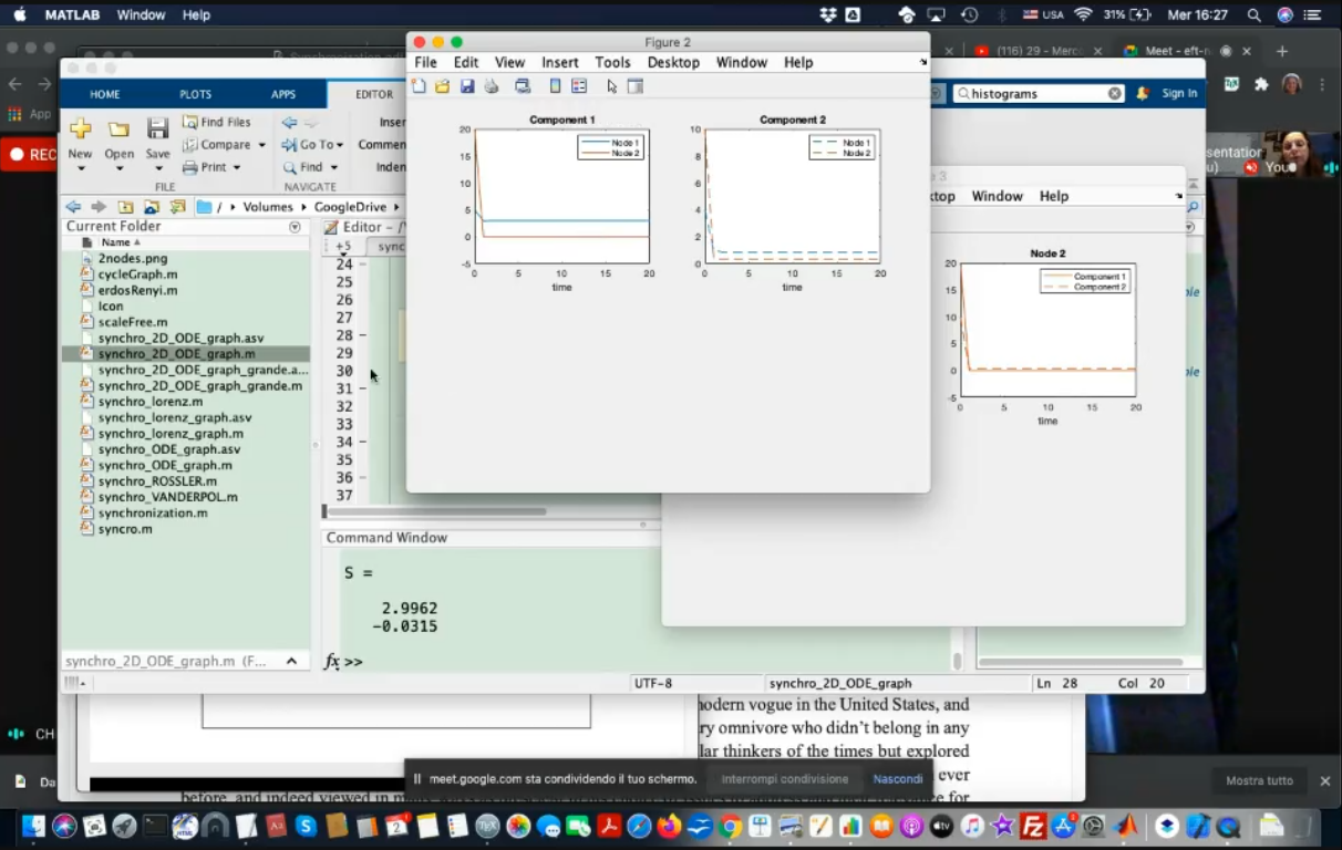
$k = 60$ , the 1st components coincide at regime, the 2nds are still different.

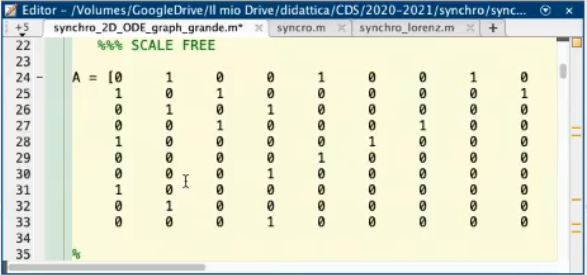
Regular large network, each node still represents a hopf bifurcation.
Some node have negative $θ$ some have a positive one.

Graph

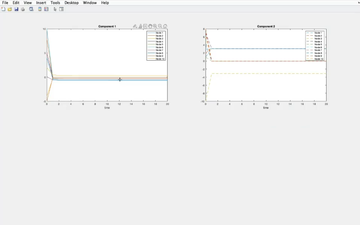
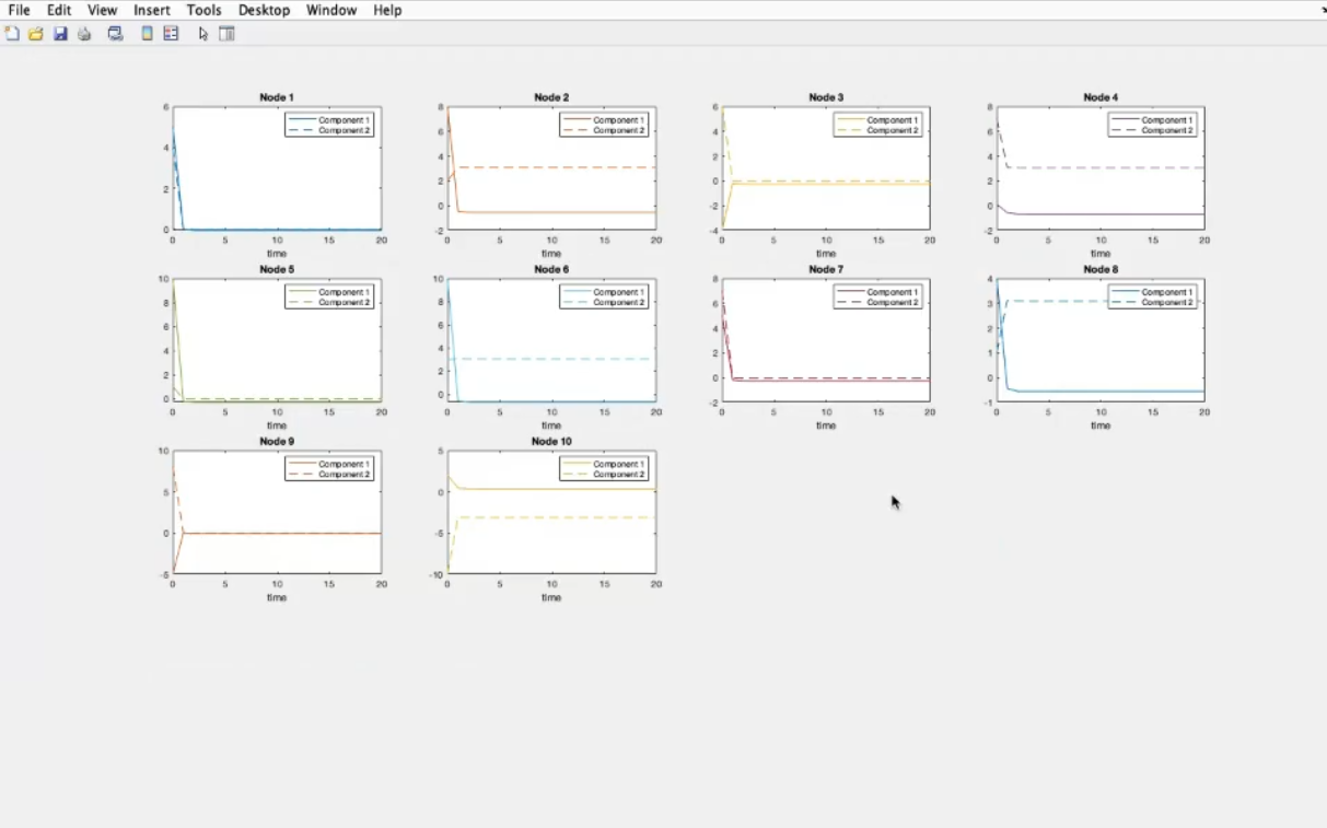
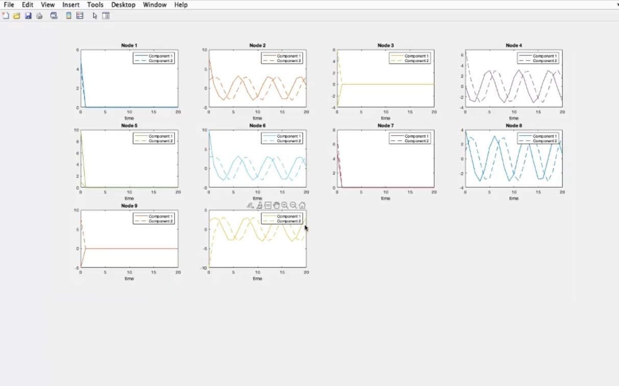
$k = 4$
The majority of them should oscillate, but as we can see the converging node help the network stabilize.

$k = 0$ (indipendente nodes)

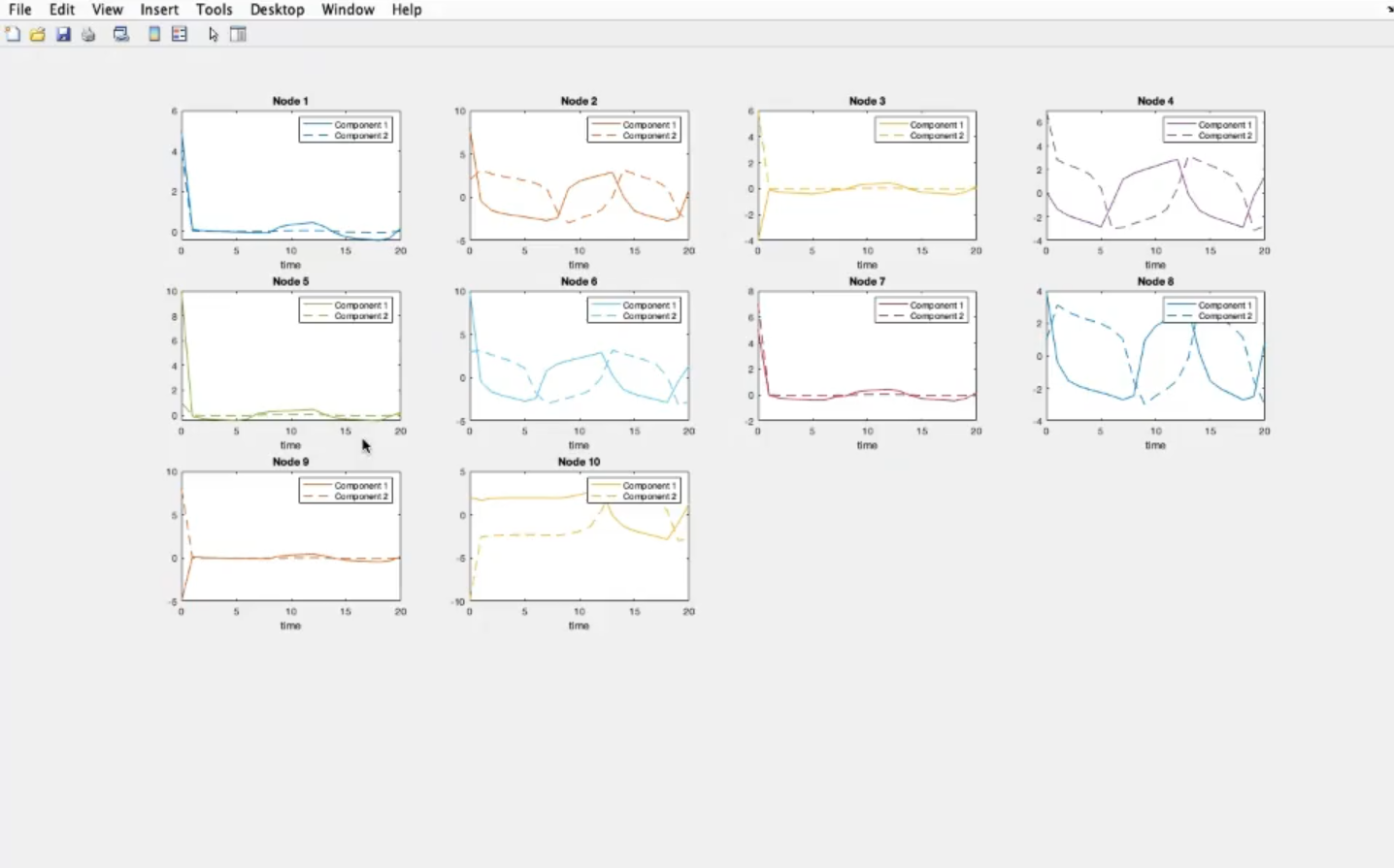
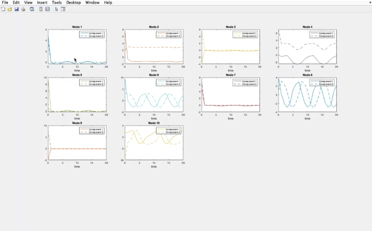
$k = 1$
They influence each other, but there is no “dominating system”.

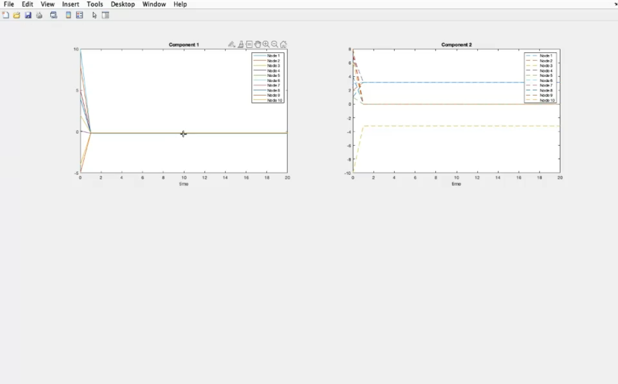
$k = 100$
The system is stabilized.

Now we change the shape of the network/graph.

Graph

$k = 0$

$k = 1$

$k = 6$
The system is syncronized.

$k = 100$
The system is stabilized.
NOTE: In this case the shape of the network does not change much about stability or syncronization, but (in general) it absolutely can.

🪴 Quartz 4.0

Explorer

CDS - Lecture 18

Graph View

Backlinks