CDS - The Lorenz System • Deterministic Chaos • Deterministic System • Sensitivity to Initial Conditions • Butterfly Effect • Lorenz Attractor • Strange Attractors

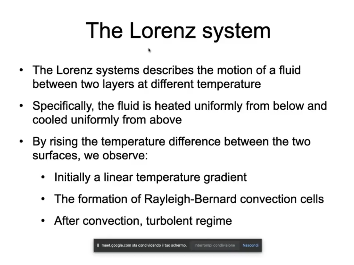
Remember:

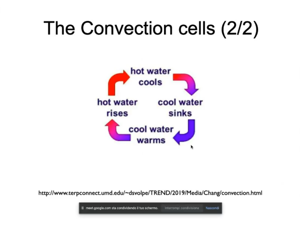
Let’s start by visualizing what happens in a bowl of boiling water, “convections cells”:
Now, we represent with the Lorenz Sysntem:

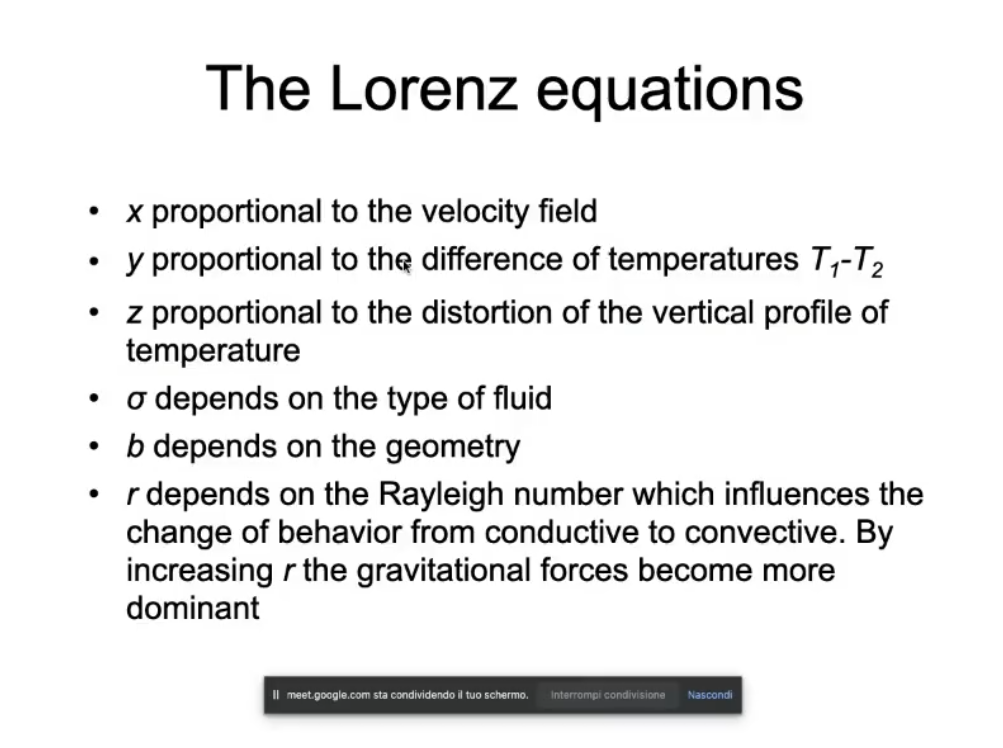
• $x$ proportional to the velocity field.
• $y$ proportional to the difference of temperatures. $\left(T_1-T_2\right)$
• $z$ proportional to the distortion of the vertical profile of temperature.
• $\sigma$ depends on the type of fluid.
• $b$ depends on the geometry.
• $r$ depends on the Rayleigh number which influences the chage of behaviour from conductive to convective.
  By increasing $r$ the gravitational forces become more dominant.

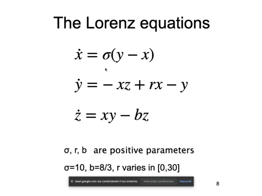
Lorenz System:$\{\begin{array}{l}\dot{x}=\sigma (y-x)\\ \dot{y}=-xz+rx-y\\ \dot{z}=xy-bz\end{array}$Where:

• $\sigma ,r,b$ are positive parameters.
  • $\sigma =10$.
  • $b=\frac{8}{3}$.
  • $r\in \left[0,30\right]$.
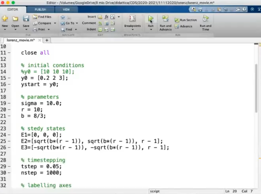
• This system is “autonomous”: no external forces influence the system.
• And it is also “almost linear”, since we only have $xz$, and $xy$ as non-linear terms.

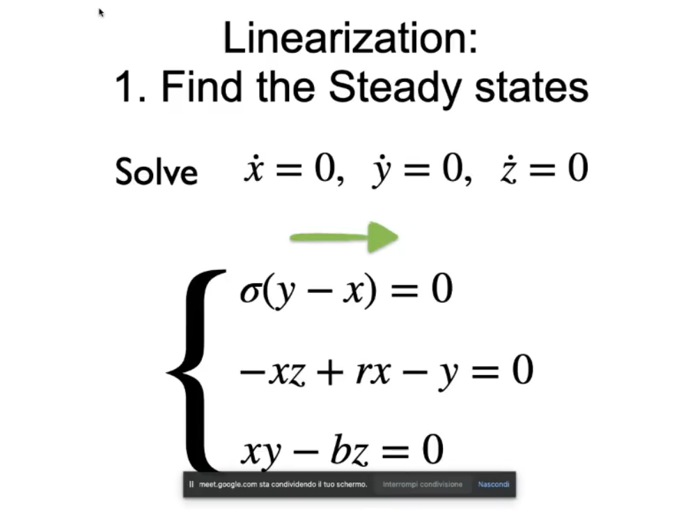
To analyze a system in general you need to:

1. Find the steady states.
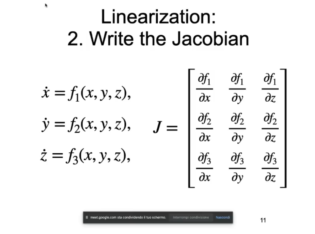
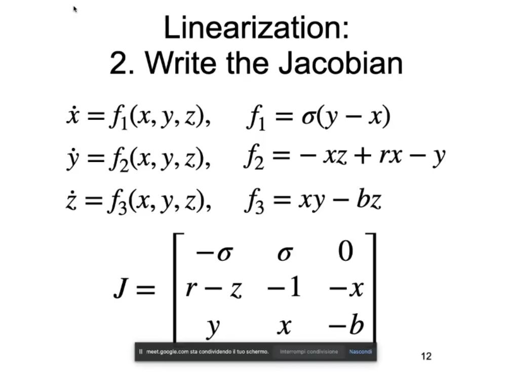
2. Linearize.
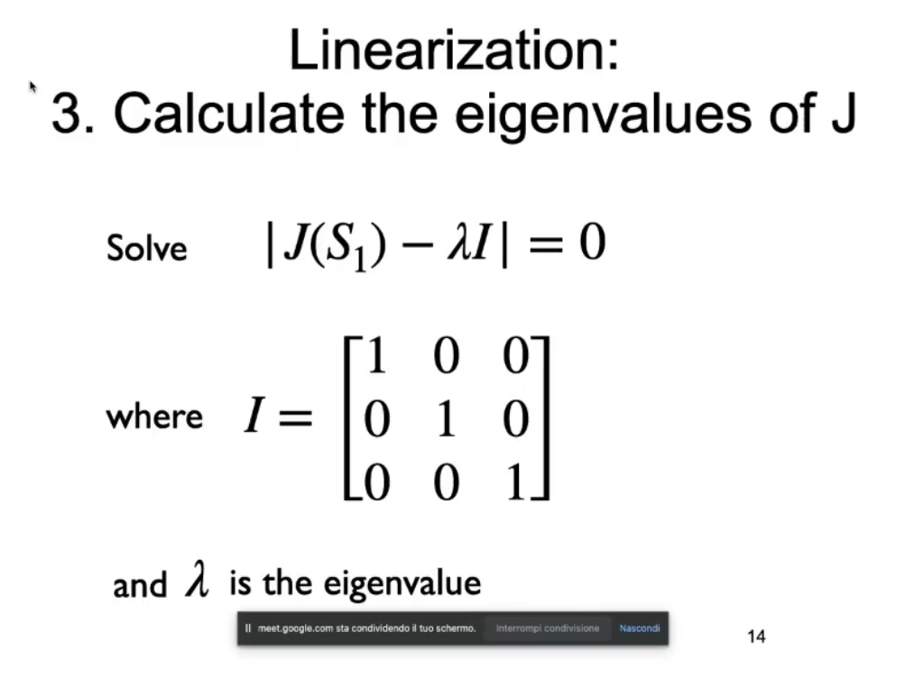
3. Substituite the steady states $S_i$ in the Jaccobian matrix $(J)$ and calculte the eigenvalues
4. Plot the Real and Imaginary part of the eigenvalues, with respect to the parameter.
5. Analyze the stability.
6. Plot the bifurcation diagram.
7. Analyze the bifurcations

1. Find the steady states:
   

• And we’ll find:$\begin{array}{l}{S}_1=\left(0,0,0\right)\\ S_2=\left(\sqrt{b(r-1)},\sqrt{b(r-1)},r-1\right)\\ S_3=\left(-\sqrt{b(r-1)},-\sqrt{b(r-1)},r-1\right)\end{array}$

2. Linearize:
   
   

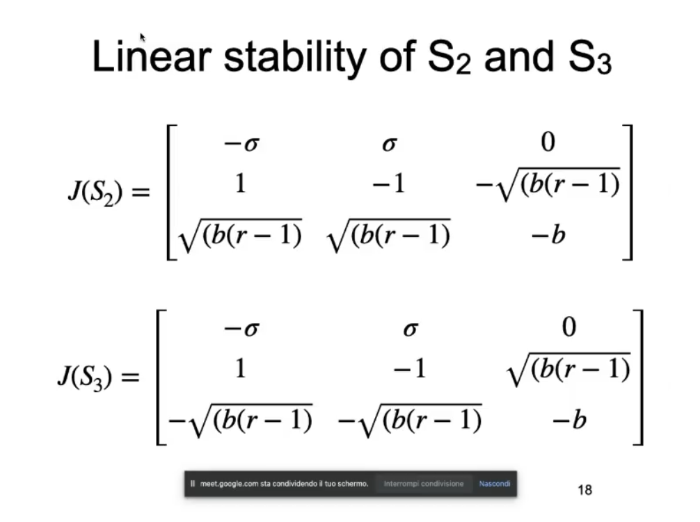
3. Substituite $S_i$ in the Jaccobian Matrix $J$ and calculte the eigenvalues:
   
   
   
   

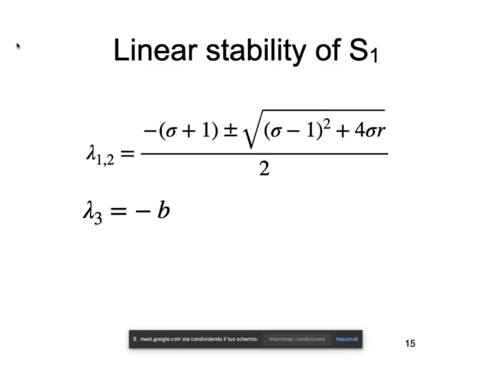
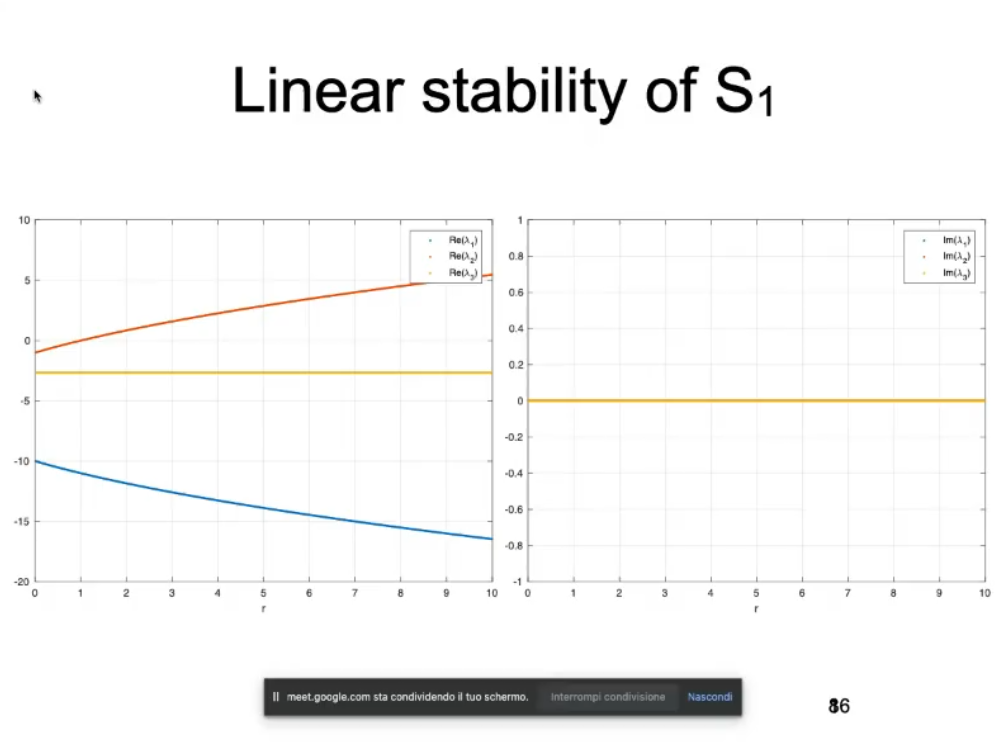
4. Plot the Real and Imaginary part of the eigenvalues, with respect to $r$.
   Rememebr that for each steady state, we have (in this case) 3 eigenvalues.
   
   

• We will analyze (and now plot) $S_2$ and $S_3$ toghter since they eigenvalues coincide.

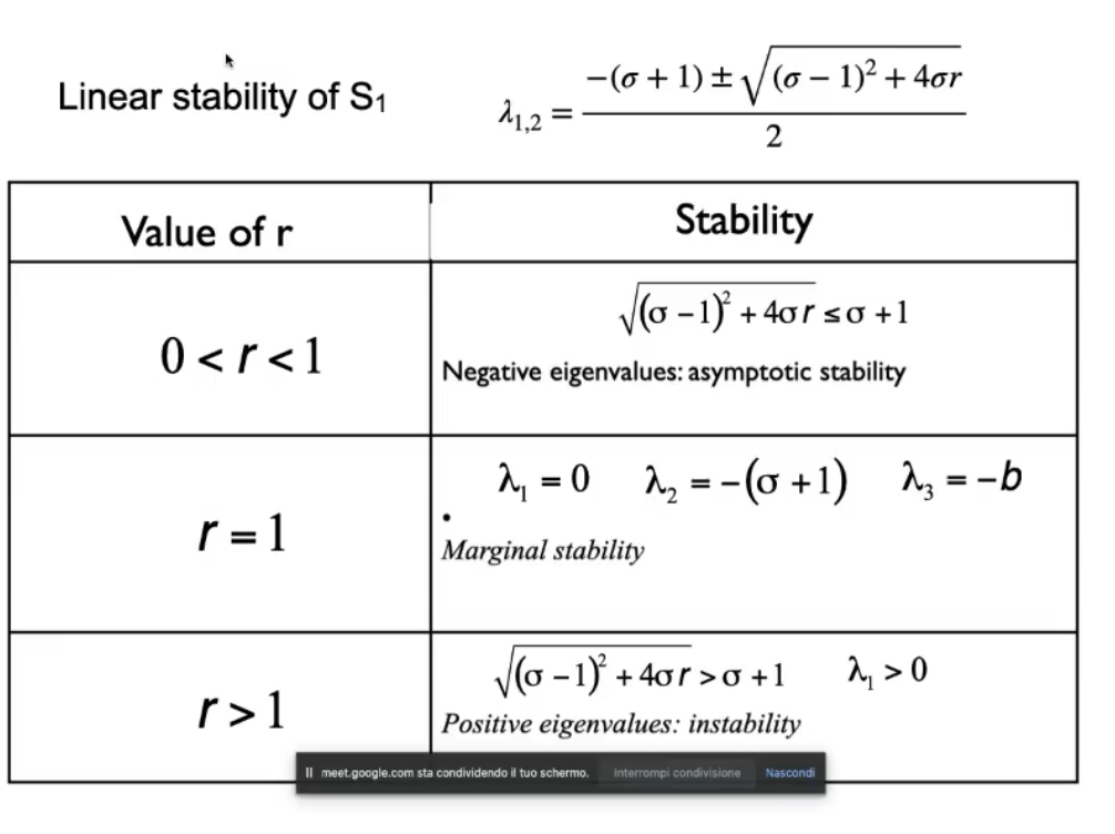
5. Analyze the stability:
   Where the real part changes sign, or more generarly the points in which the real part the eigenvalues beomes zero, for each steady state:
   
   

• $r_H\simeq 24.74$ (called “critical value”) found using MATLAB.

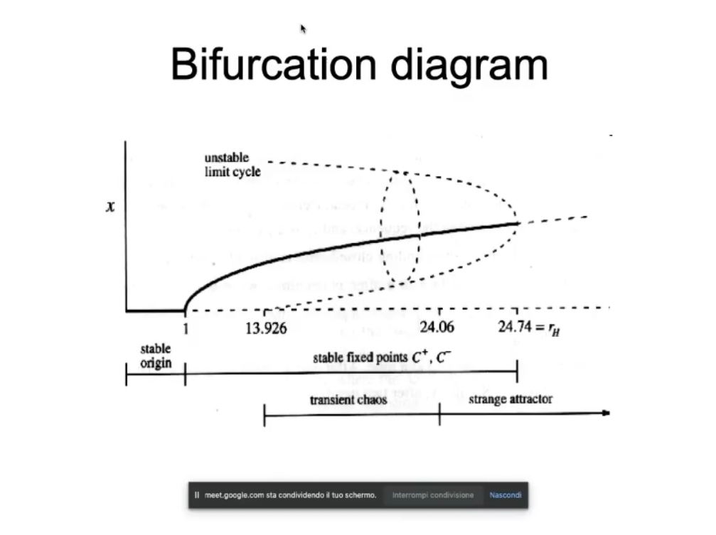
6. Plot the bifurcation diagram:
   

• We don’t see in this picture but there is another unstable limit cycle mirrored with respect to the abscissa.
• NOTE: above $r_H$ we have no stability exist/no attractors.
  Unstable for the linearization ⇒ unstable for the real system.

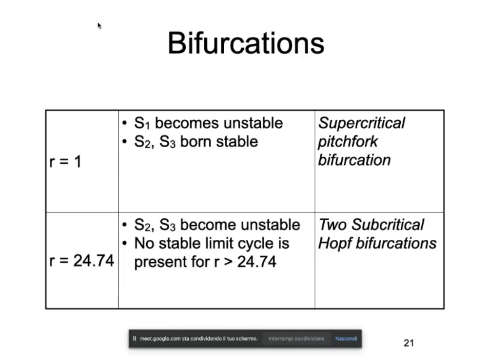
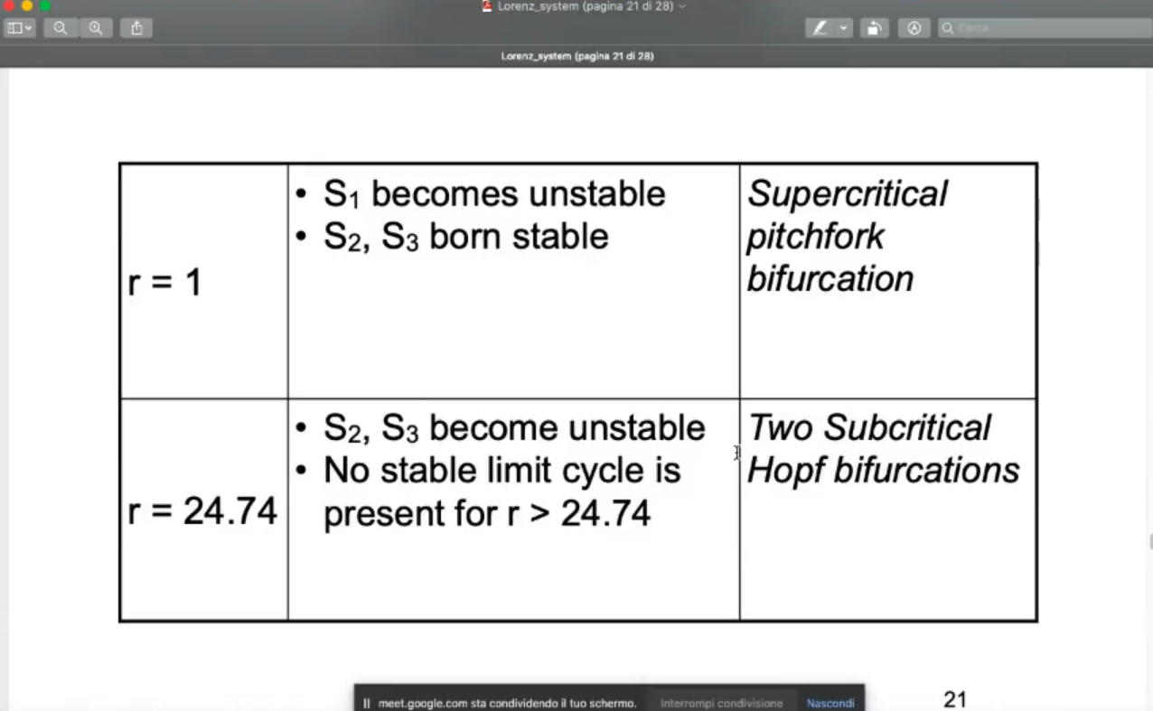
7. Analyze the bifurcations:
   Let’s give a name/type for this bifurcations
   

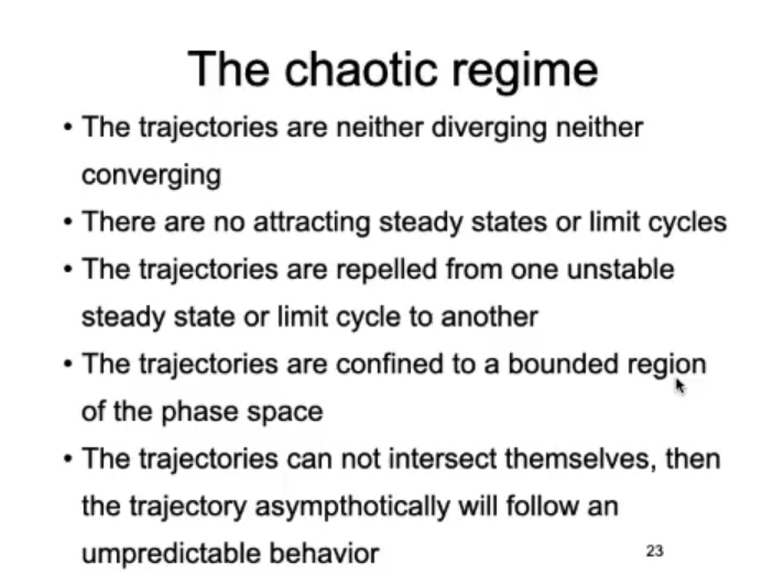
Now we define the chaotic regime for the Lorenz system, and try to understand what is happening:

• The trajectories are neither diverging neither converging.
• There are no attracting steady state or limit cycles.
• The trajectories are repelled from one unstable steady state, or limit cycle to another.
• The trajectories are confined to a bounded region of the phase space.
• The trajectories cannot intersect themselves, then the trajectory asympthotically will follow an umpredictable behaviour.

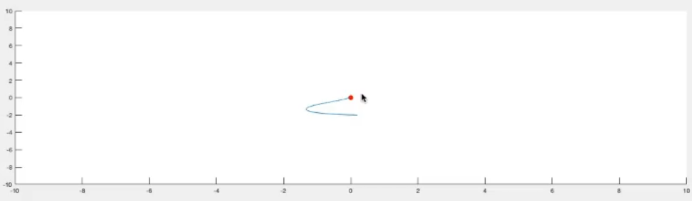
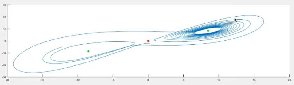
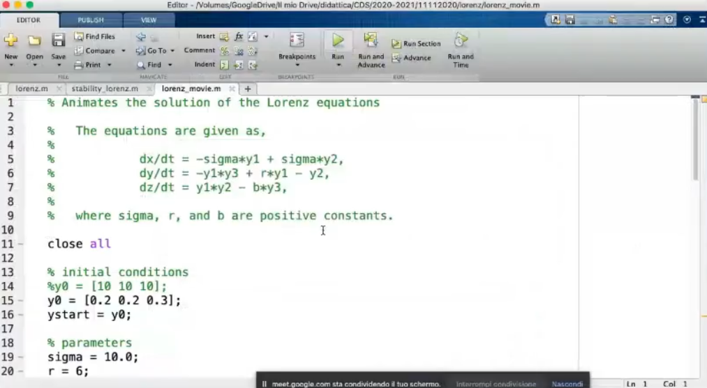
Here is the Lorenz system for $r<1$:

Here is the Lorenz system for $r\in (1,r_H)$. given two diffrent initial conditions:

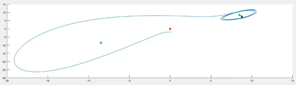
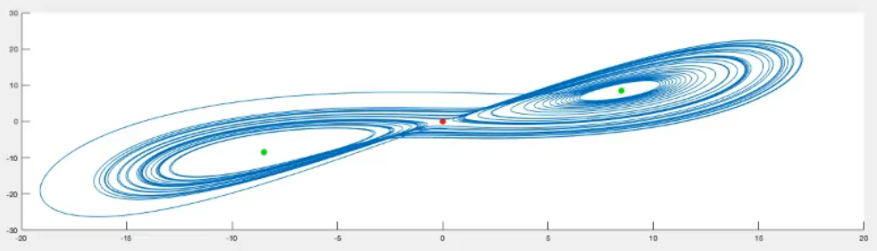
Instead if we take $r>r_H$ then we are in the chaotic regime, let’s see how the phase space evolves in time:

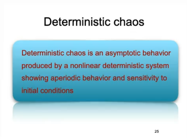
Definition ‘Determinstic Chaos’: There is no formal definition of “chaos”, these are its properties. Deterministic chaos is an asymptotic behaviour produced by nonlinear deterministic systems, showing aperiodic behaviour and sensitivity to initial conditions*. A chaotic system is deterministic and presents sensitivity to initial conditions.

Defintion ‘Deterministic’: *Given an initial condition, we have an unique solution.

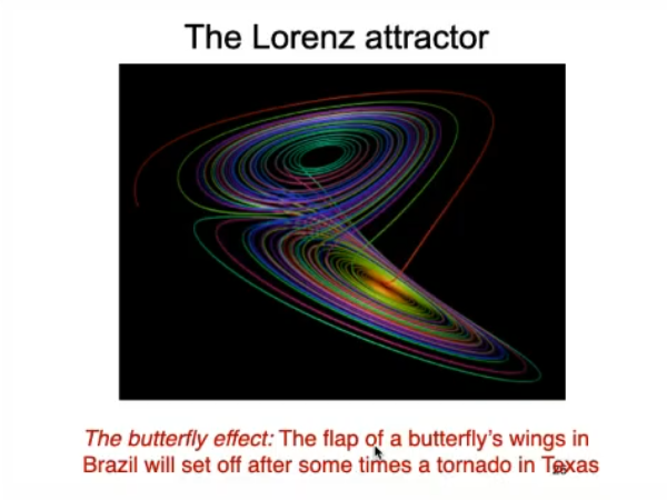
Defintion ‘Sensitivity to Intial Conditions’: This is also called the “butterfly effect”: A very very tiny change of the inital conditions, will produce an enormous change in the system after some time.

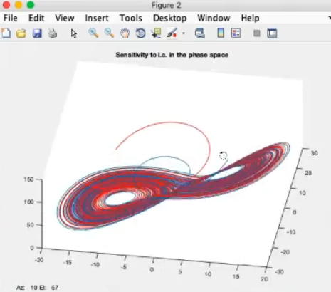
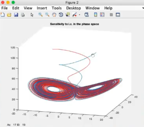
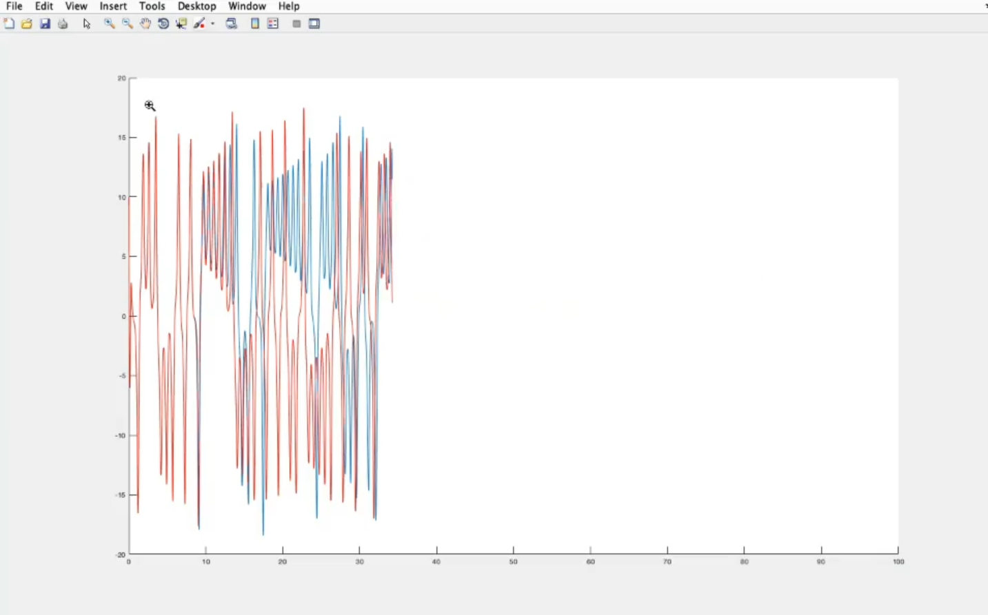
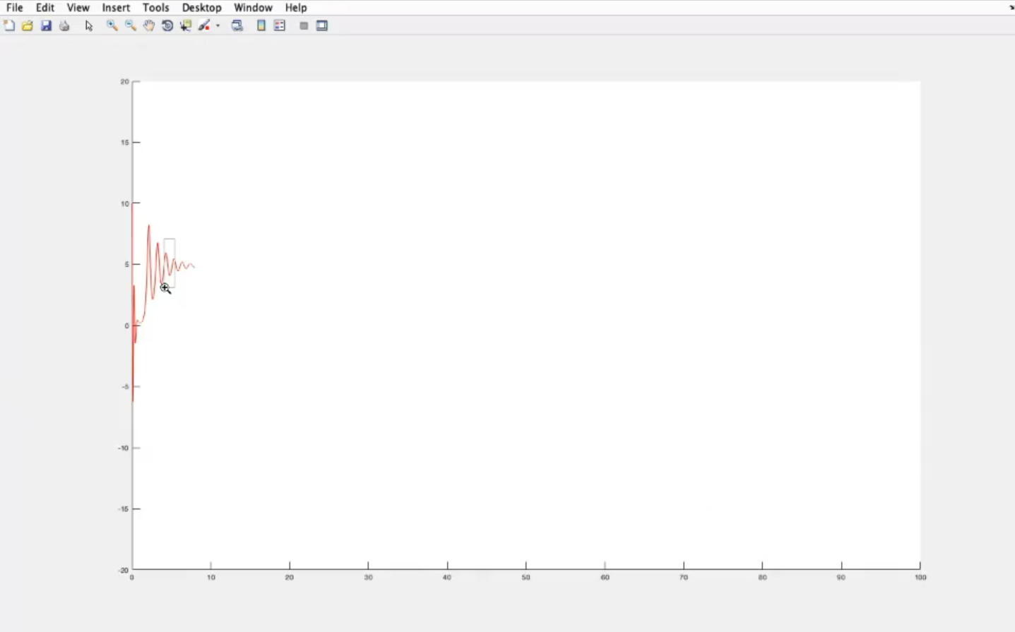
Graphical representation of sensitivity to intial conditions, take the Lorenz system, in the chaotic regime (so: $r>r_H$), and take two intial condtions (we will see them represent in blue and in red) extreamely close to one another, this is what happens for a chaotic system, specifically this is the graph of a sysmtem that has sensitivity to intial conditions:
As you can see the two variables become compleately different after some time, even if they started really close to one onother.

Definition ‘Lorenz attractor’: It is called an attractor, since the system will not diverge, it will remain confined in a closed region. It is also called “strange attractor”, because ins not a typical one, the typical one are:

• stable steady states (atttractors)
• limit cycles (and multiple-period limit cycles)

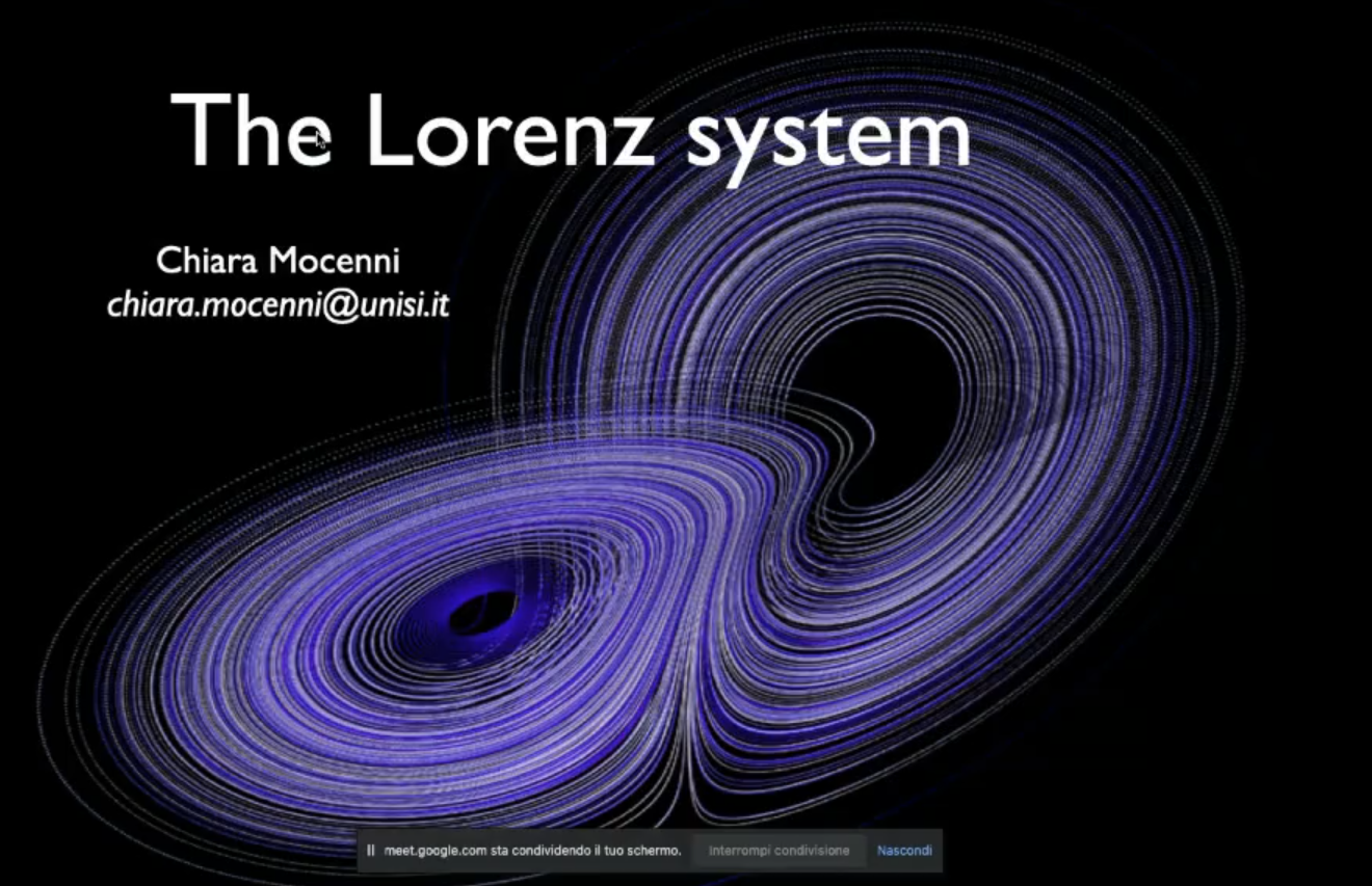
The Lorents system, 3D graphical representation
:

---

• $T_1>T_2$
• This is a somewhat of an “organization” (not compleately chaotic).

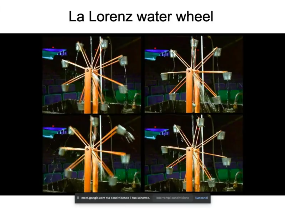
• The four weels will evolve differenty (sensitivy to inital conditions)

• Autonomous (no external forces influence the system)
• Almost linear (we only have $xz$, and $xy$ as non-linear terms)
• We fix $\sigma$ and $b$ and study the system for $r\in \left[0,30\right]$.

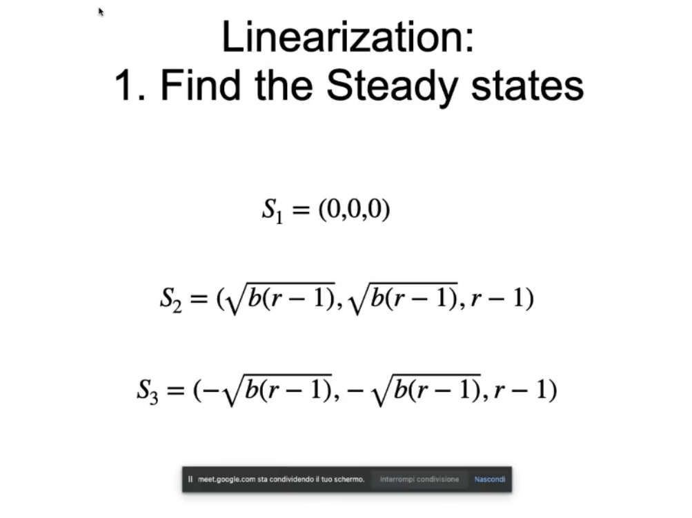
• We find $3$ steady states.

• Remeber that “linearization is a local process”, so we’ll need to repeat the following process for each steady state.

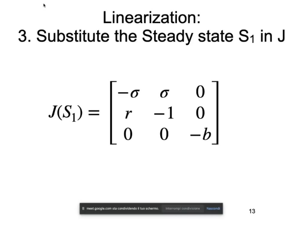
• Remeber that: $S_1=\left(0,0,0\right)$

• bifurcation diagram.not-sure-about-this

• Remeber that: $S_2=\left(\sqrt{b(r-1)},\sqrt{b(r-1)},r-1\right)$
• Remeber that: $S_3=\left(-\sqrt{b(r-1)},-\sqrt{b(r-1)},r-1\right)$

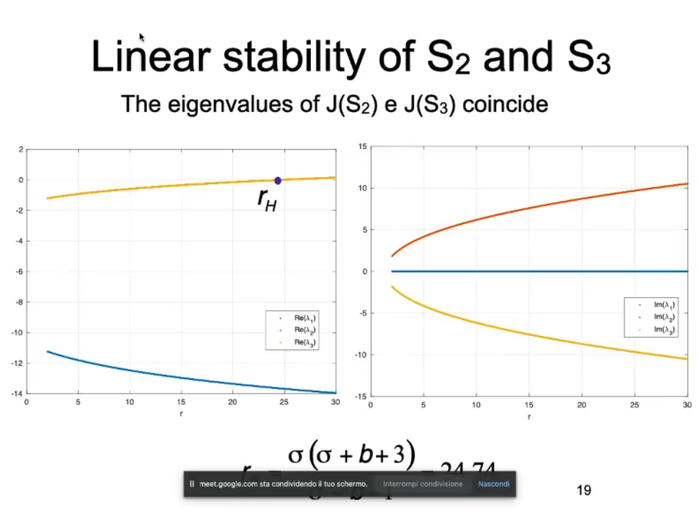
• The have non-zero imaginary part.
• For $r\in \left[1,\sim 24.74\right]$ the real parts of the eigenvalues are negative.
• $\mathrm{Re}({\lambda }_1)=\mathrm{Re}({\lambda }_2)$.
• For $r<r_H$ (called “critical value”) then the system is stable.
• For $r>r_H$ the system is unstable.
• For $r=r_H$ the real part of the 3rd eigenvalue $\mathrm{Re}({\lambda }_3)=0$.
• $r_H\simeq 24.74$ found using MATLAB

• We don’t see in this picture but there is another unstable limit cycle mirrored with respect to the abscissa.
• NOTE: above $r_H$ we have no stability exist/no attractors.
  Unstable for the linearization ⇒ unstable for the real system.

• $r=0.4$.

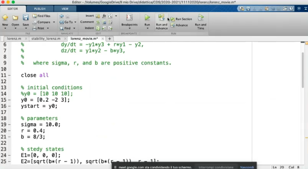
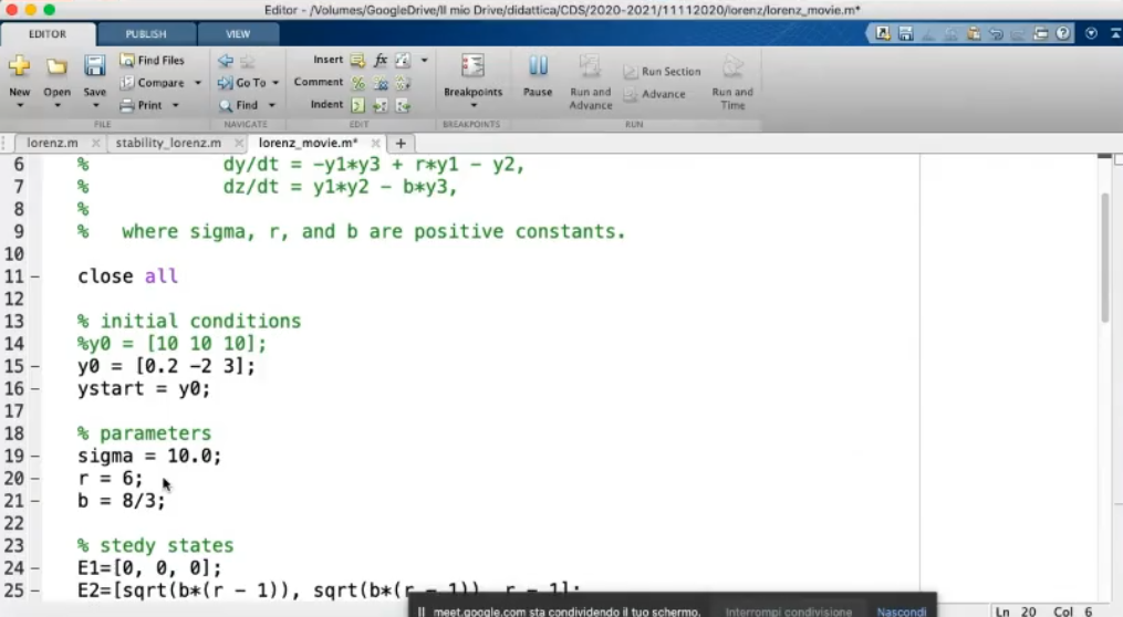
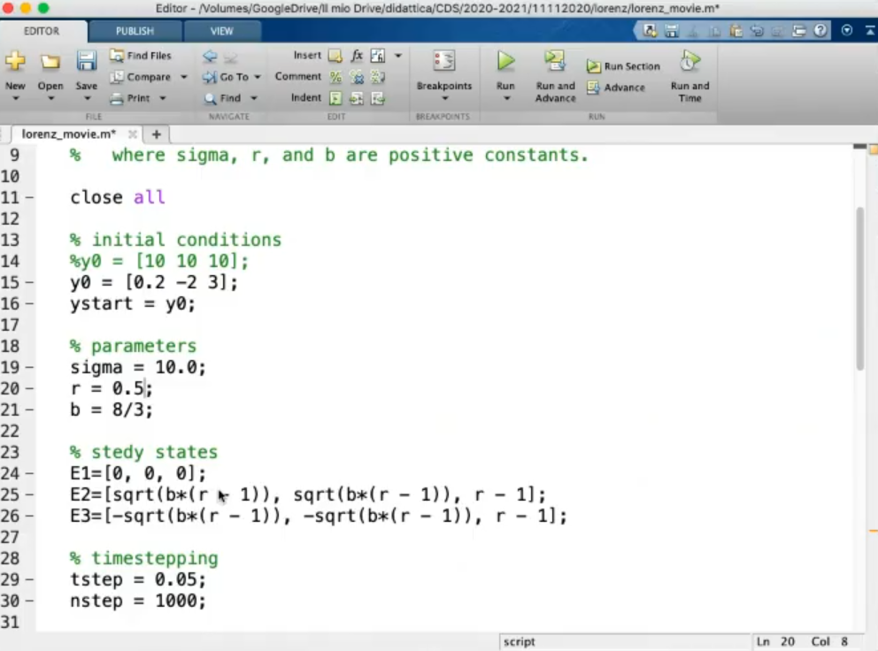
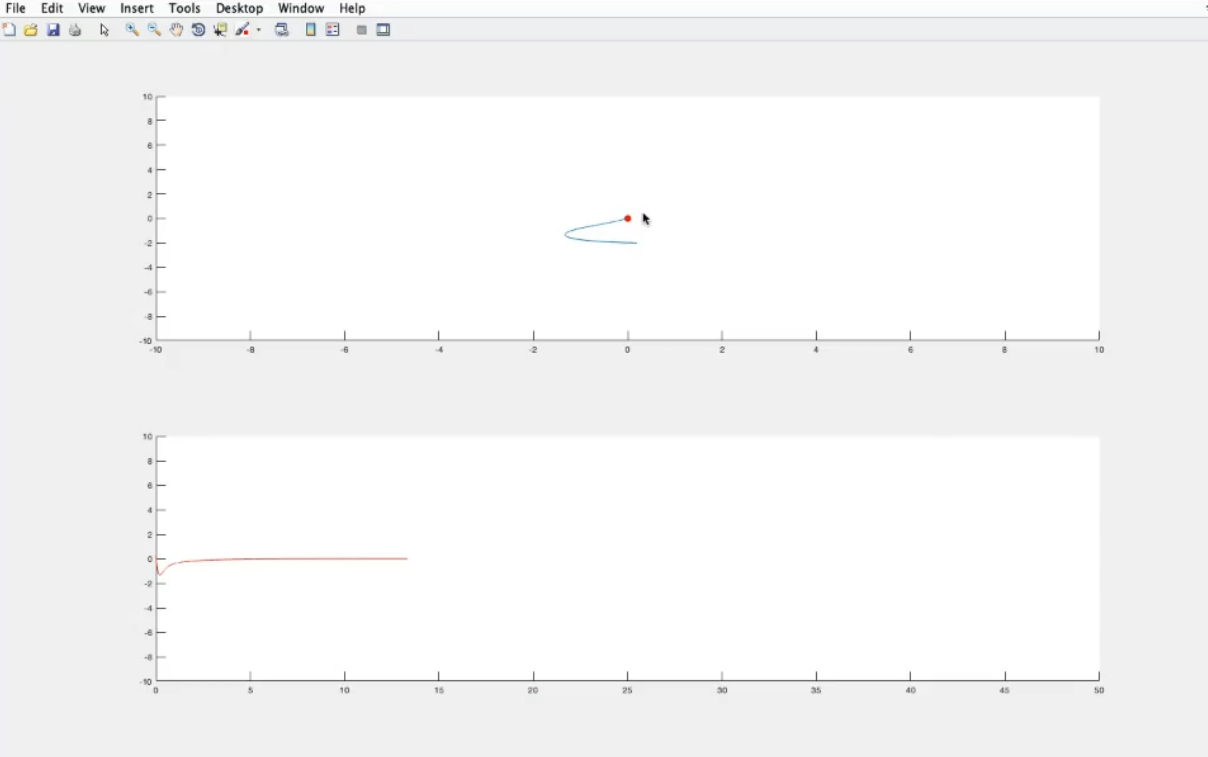
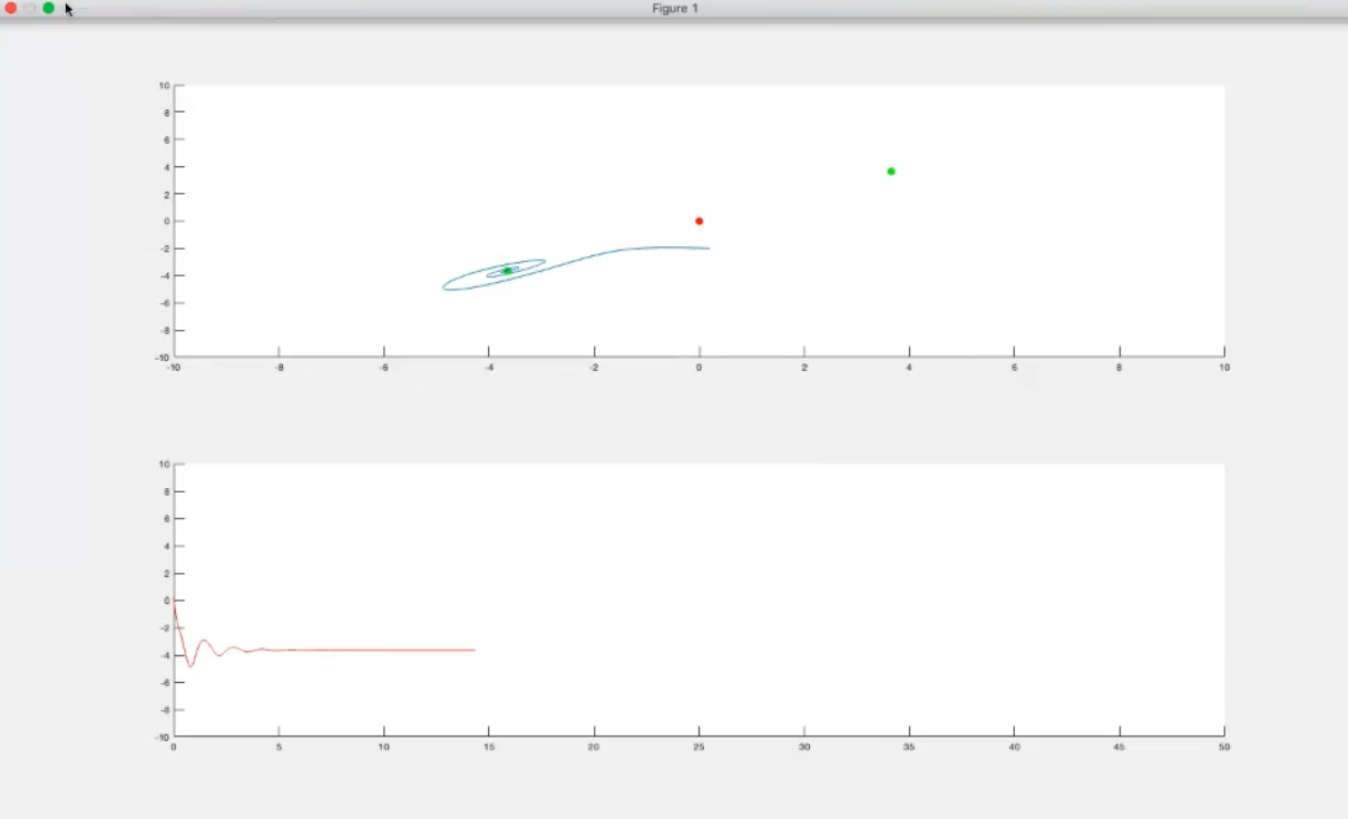
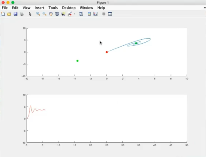
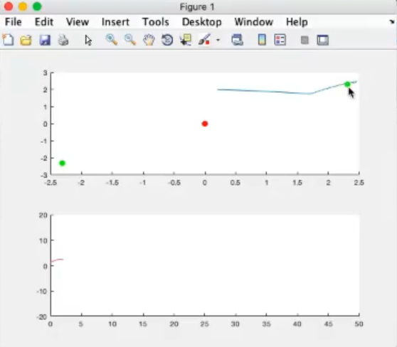
• Output of the previous, code:
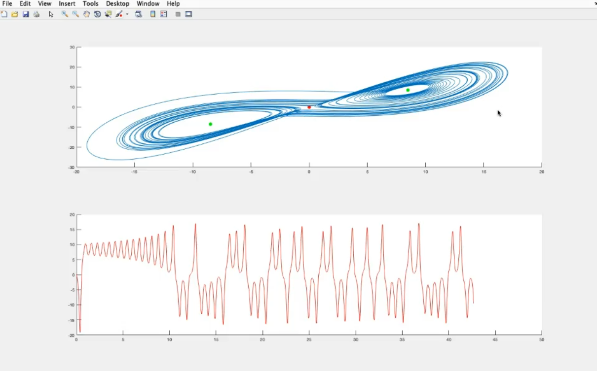
  • In the first subplot we represent the phase space.
  • In the second subplote we represent the dynamics.

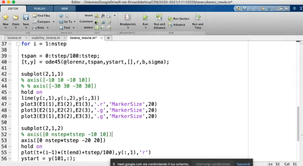
• $r>1$ (specifically $r=6$)

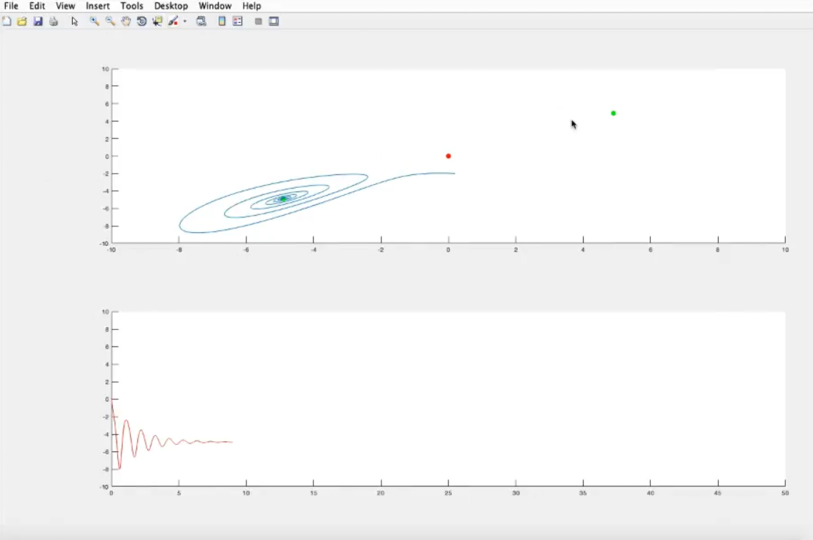
• Output of the previous, code.
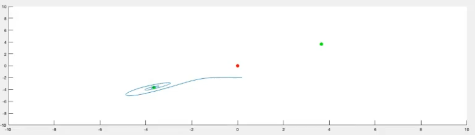
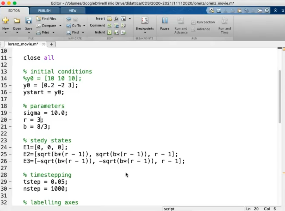
• The origin is now an unstable steady state

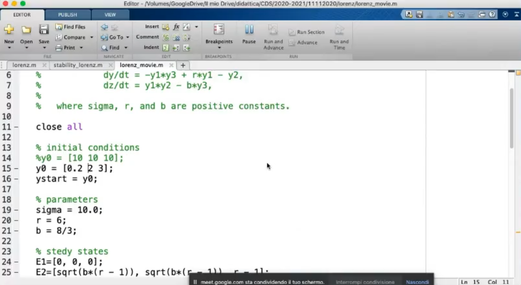
• We change the initial conditions, $y_0=\left[0.2,2,3\right]$

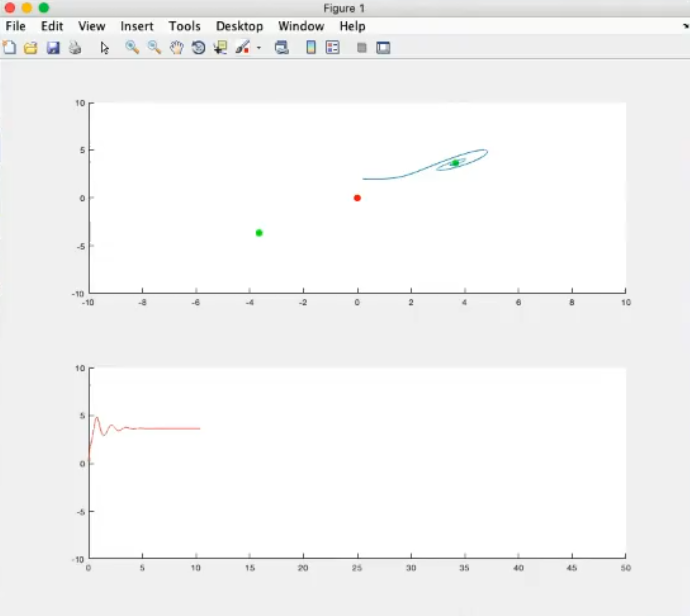
• We now converge to the second stable steady state.

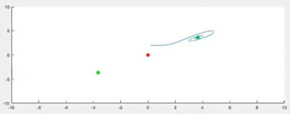
• We change the initial conditions, $y_0=\left[0.2,0.2,0.3\right]$ (closer to the origin)

• $r=10$.

• $r>r_H$ ($r=28$)

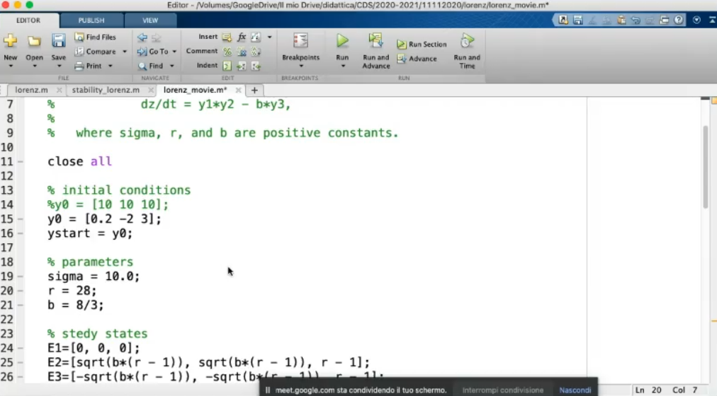
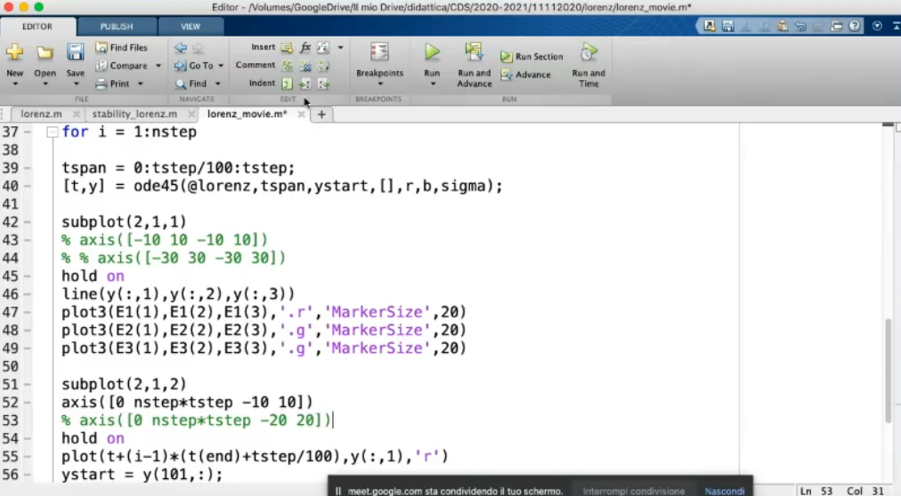
• Also we change the scale of to the abscissa and ordinate.
• (comment axis([0 nstep*tstep -10 10]))
• (uncomment axis([0 nstep*tstep -20 20]))
• (comment axis([-10 10 -10 10]))

This is the evolution of the chaotic system: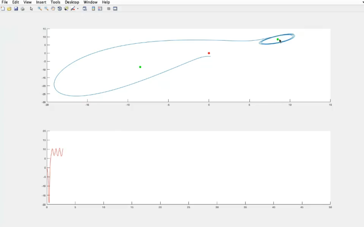

• Sensitivity to inital conditions, we report only one varible ($x(t)$), and 2 sliglty different initial conditions, as you can see they become compleately different after some time, even if they started really close to one onother.

• A very very tiny change of the inital conditions, will produce an enormous change in the system after some time.
• It is called an attractor, since the system will not diverge, it will remain confined in a closed region.
• It is also called “strange attractor”, because ins not a typical one, the typical one are:
  • stable steady states (atttractors)
  • limit cycles (and multiple-period limit cycles)

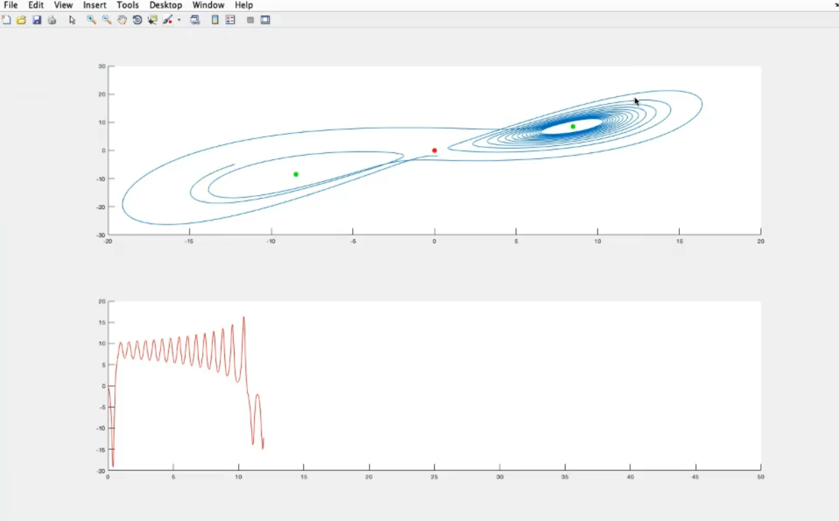
Rememebr that this is a 3D object: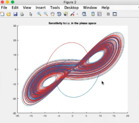

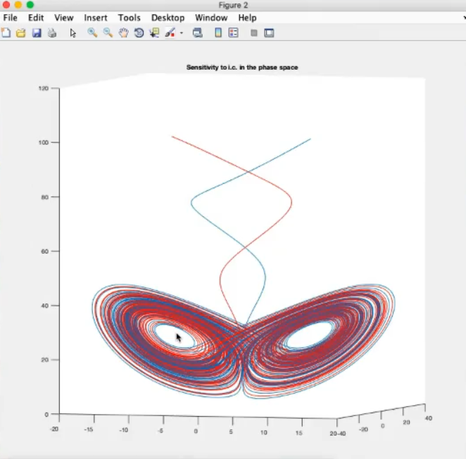
• The two circles are unstable steady states.
• In the middle of the two unstable steady states we have the origin $\left(0,0,0\right)$.

• $r=0.5$

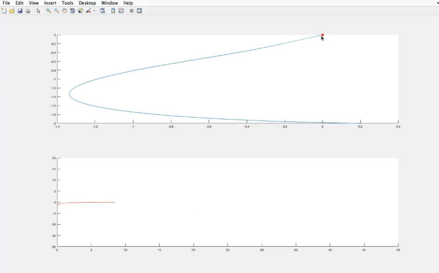
• The red point is the origin, and also an attractor steady state.

• $r=3$

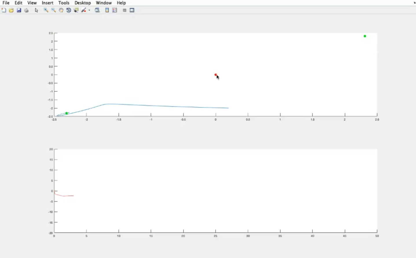
• The origin is now a non-stable steady state.
• Two attractive stable steady states appear.
• Depending on the inital conditions, the system converges to one of the two steady states:
  

• $r=10$
• … same as CDS - Lecture 12

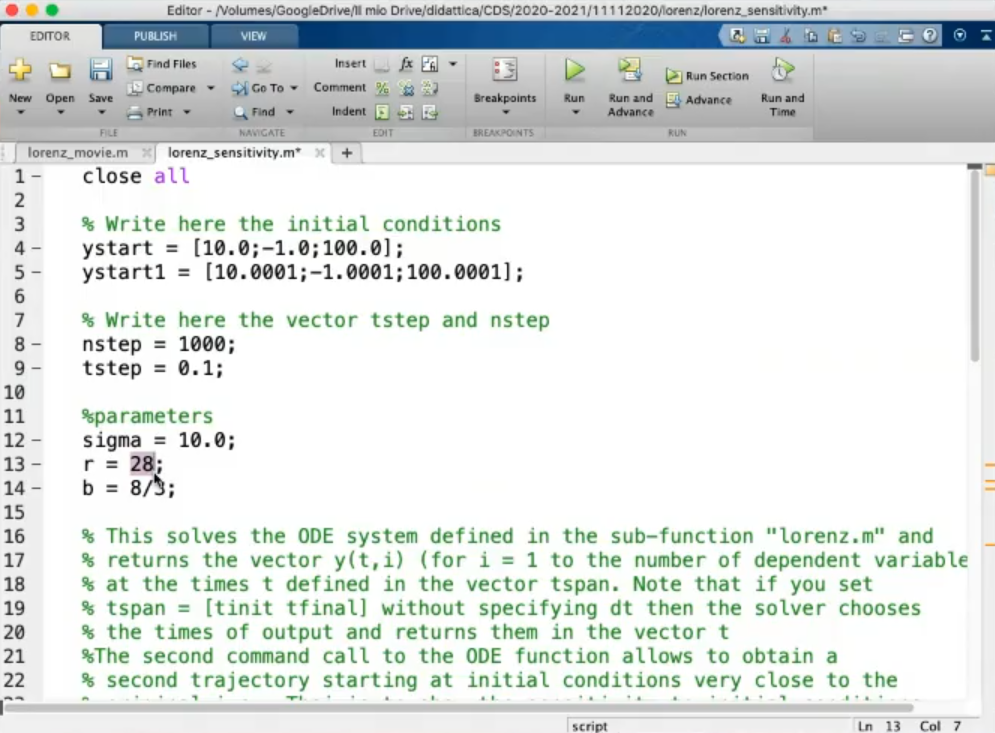
• For $r>r_H$ the system is chaotic.
• Here’s the sensitivy to intial conditions, we change the inital condition of about $0.001\%$, and the results are completly different after some time.

• NOTE: this is true only for $r>r_H$ (so we are in the chaotic regime), otherwise if we are in a stable or unstable “region”/“regime” the system will be the same (a stable/ustable system has no sensitivy to intial conditions)
• If we change the $r$ to $r=10$ this will be the resuts (the two graphs coincide so we can only see one):
  
  If we zoom (a lot):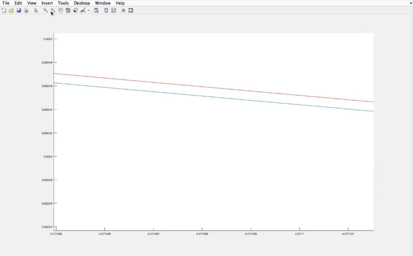
  

• There is no formal definition of “chaos”, these are its properties
• Deterministic: “*given an initial condition, we have an unique solution”.