CDS - Saddle-Node Bifurcation

Remember:

Saddle-Node Bifurcation:

• First we have a stable and an unstable steady states, so a saddle
• Then they both converge to a single point, a node.
• Finally both steady states disappears.

~Ex.:

---

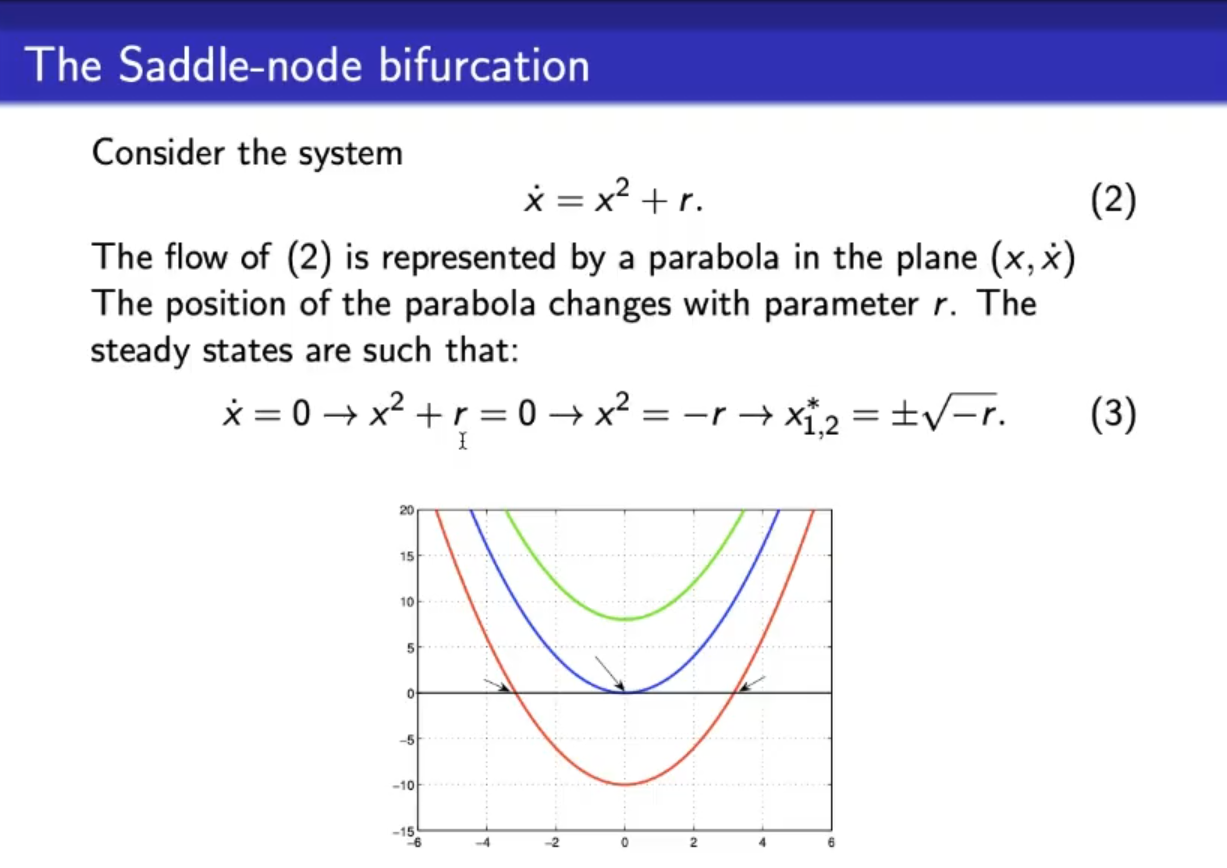
• This graph is NOT the “bifurcation diagram”, we will see it later.
• The arrows in the diagram represnt the steady states, depending or $r$ we may have $2$, $1$ (actually $2$ “coinciding” steady states) or $0$ steady states.
• If we analyze this steady states, like we have seen in the previous lectures, we can see that (looking at the red curve), we have 1 stable ss and 1 unstable ss.

• So for $r=0$ we have a bifurcation.
• Also not that for $r=0$ we have a marginal system/we are in a marginal systuation.
  You can imagine the two steady states (for the red curve, that are 1 stable and 1 unstable) uniting giving un a mix between a stable and unstable ss, however this does not mean that it’s a marginal ss, more on that later.

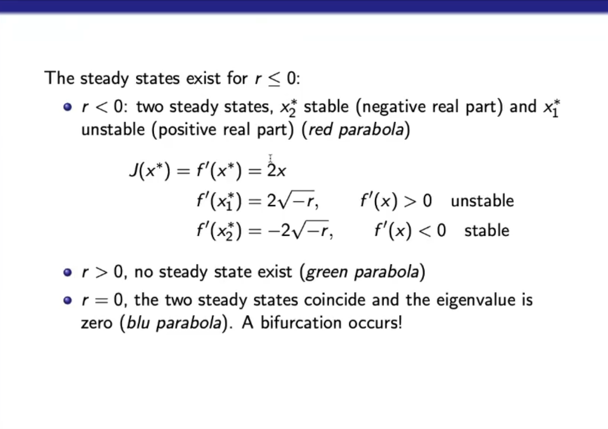
Let’s see how we analyzed the steady states on the red parabola: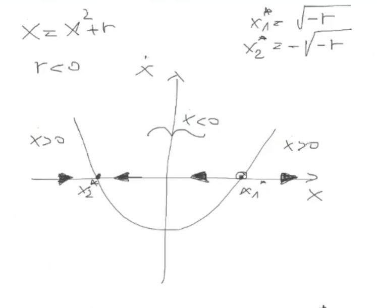
If we perform the linearization:

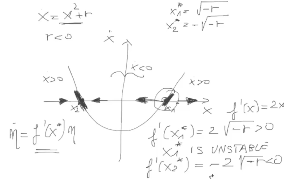
REMEMBER: in a non-linar system you may have no steady state, while in a linear system you have at least 1 ss.

For 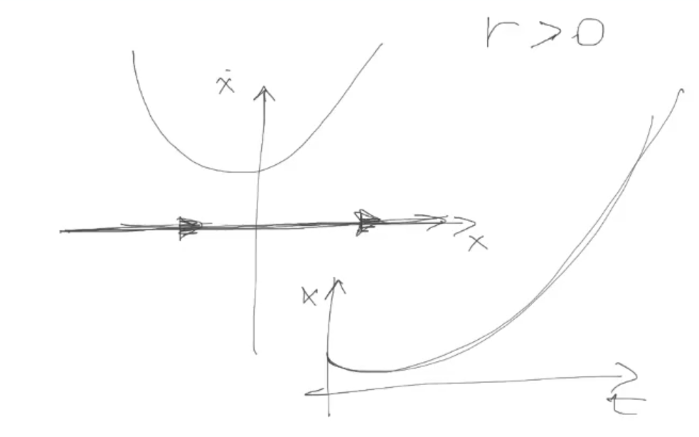$r>0$:
We have no steady states.

For $r=0$, the approximation is marginally stable: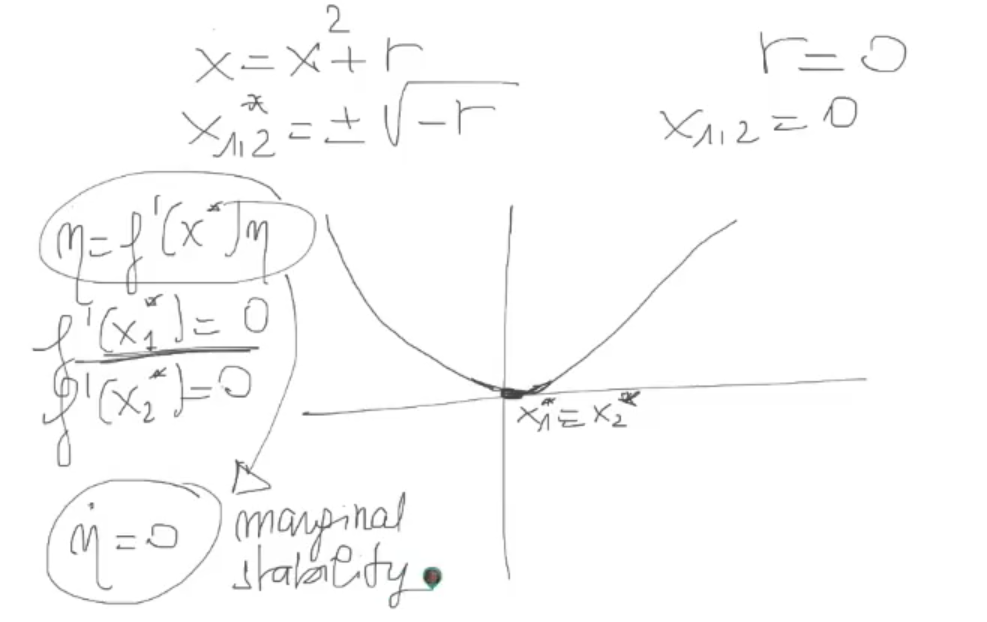
But the actual steady state is NOT!:

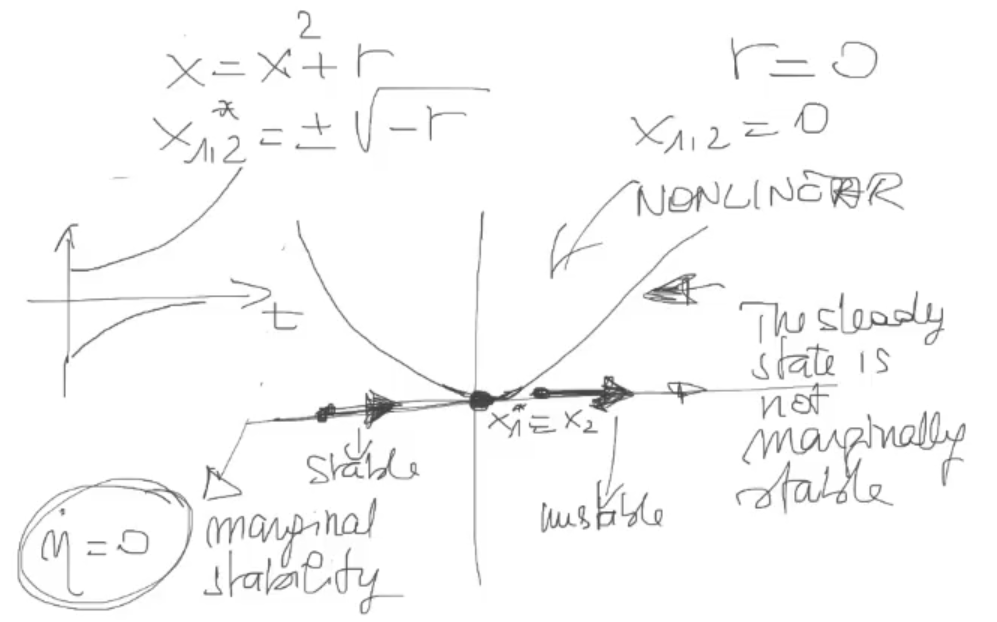
• If we take an inital condition on the left $(x<0)$ than we will have a stable system.
  However it we take an inital condition on the right $(x>0)$ than we will have an unstable system.

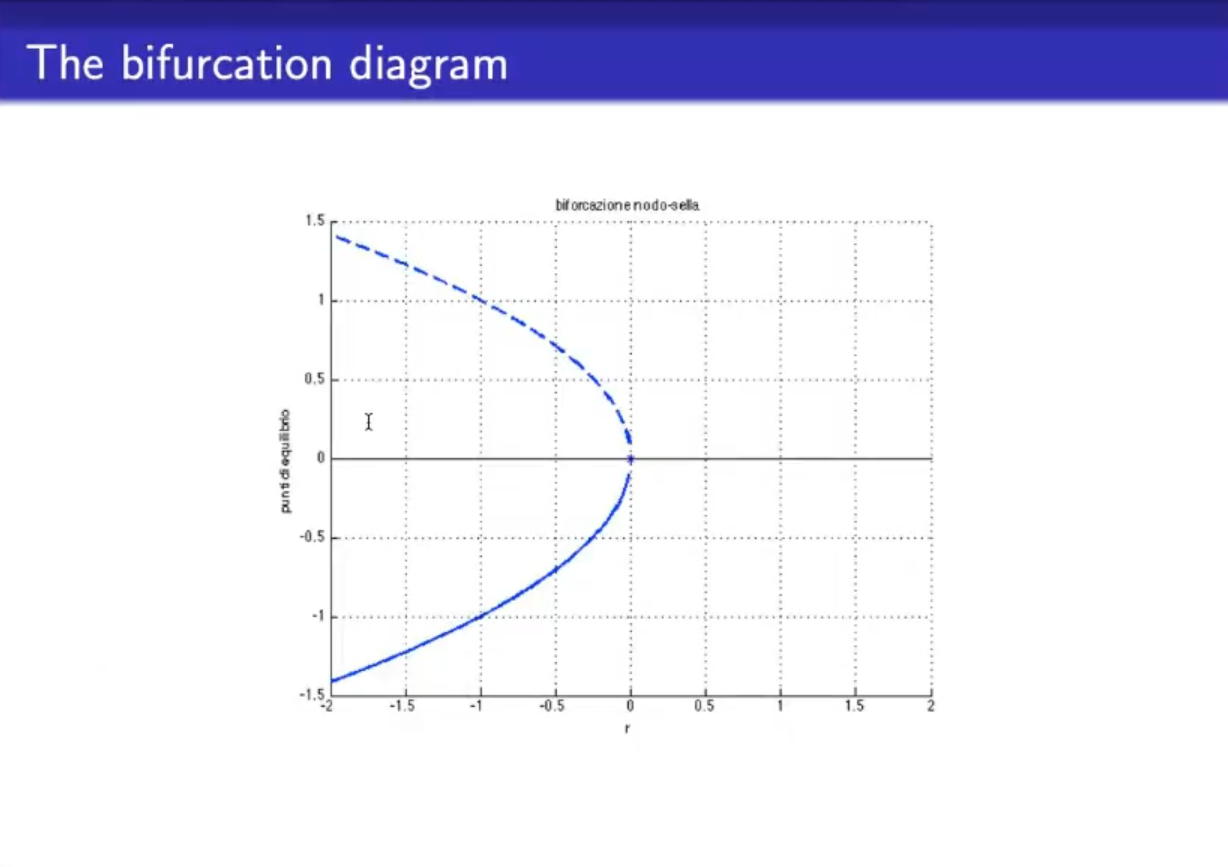
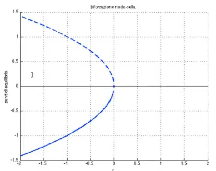
• This is the “bifurcation diagram”.
• The x-axis represents the values of the parameter $r$.
• The y-axis represents the values of the steady states.
• A continuos line represents a stable ss.
• A dotted line represents an unstable ss.
• For $r=0$ we have a bifurcation, and specifically this is a “saddle-node bifurcation”, since we have 1 stable and 1 unstable steady states that collpase.