CDS - Lecture 5

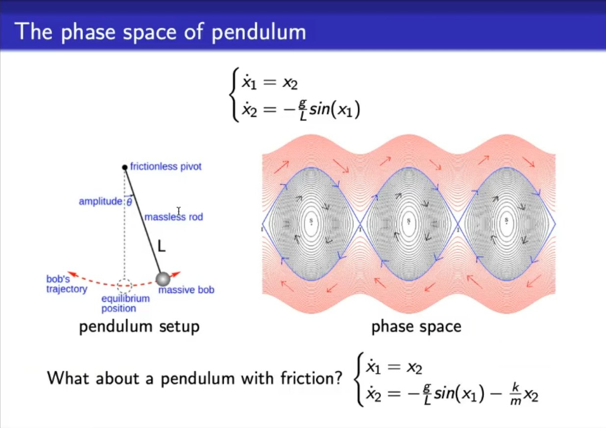
• Pendulum example, we do not account for friction, so it will continue to move endlessly.
  • For this system: $x_1$ represents the position, $x_2$ reperesents the velocity.not-sure-about-this
• The system has two steady states, one unstable, when the pendulum is held with muss “up”, and one marginally stable ss when the mass in the “equilibrium position”, it is marginally stable because this system does not account for friction.
  • The marginally stable steady states are represented in the phase space with the “s” (look a the point inside the black lines)
  • While the unstable steady states are represeted with a “i” (look at the intersection of the blue lines with the $x_1$ axis)
• In the phase space:
  • The black circular lines indicate: when the pendulum oscillates (not enough initial velocity for a complete rotation)
  • The red lines indicate: when the pendulum compleately rotates, however notice that the velocity of the pendulum never reaches $0$.
  • The single blue line indicates: this is a special case in which the pendulum actually stops $(x_2=0)$ in the upper point, also note that for the exact initial conditions such that we begin with the pendulum in one of the “i” unstable ss, then it will not move (it is a ss after all).
• When you add friction the phase space changes such that the marginally steady states, now become stable steady states, and the flows will all reach this state, with enough time.

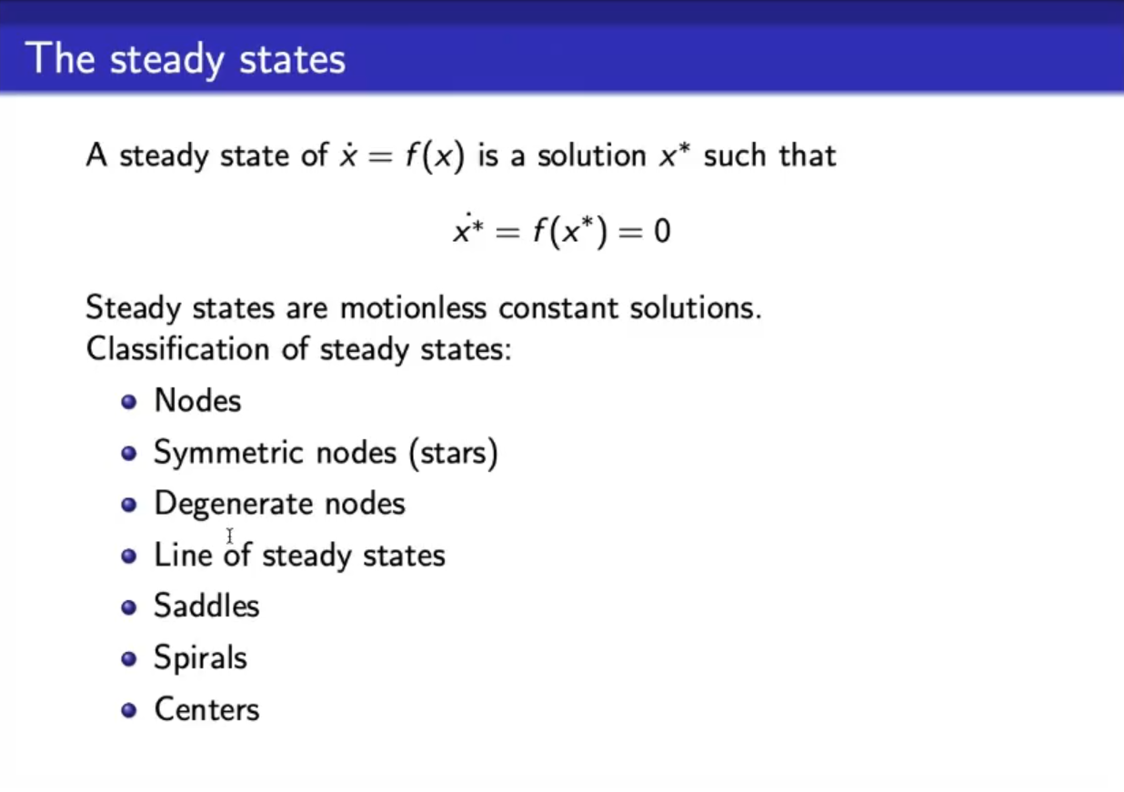
• Remeber that $x$ is a vector, in the previous case: $x=⟨x_1,x_2⟩$, so we need to find the solutions $x^{\ast }=⟨x_1^{\ast },x_2^{\ast }⟩$ such that:$\{\begin{array}{l}{x}_2^{\ast }=0\\ -\frac{g}{L}\sin (x_1^{\ast })=0\end{array}$

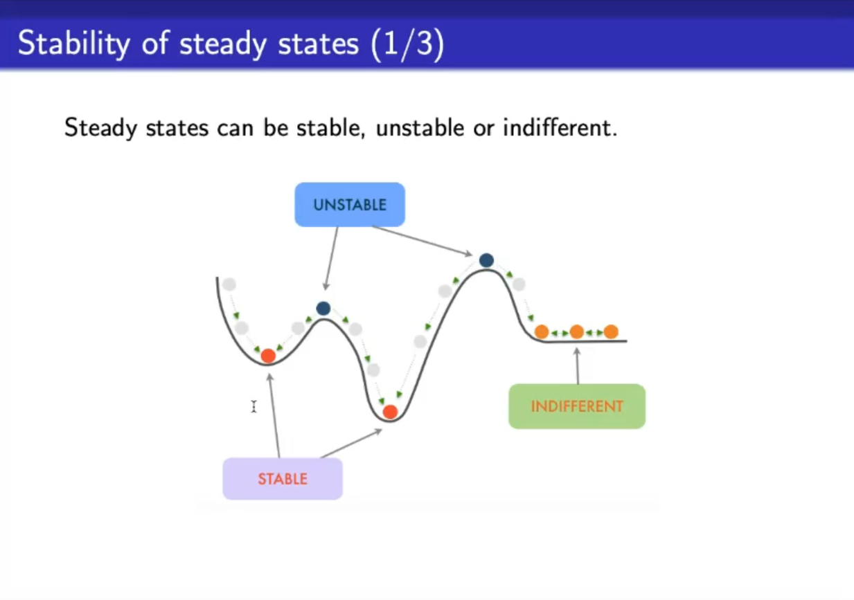
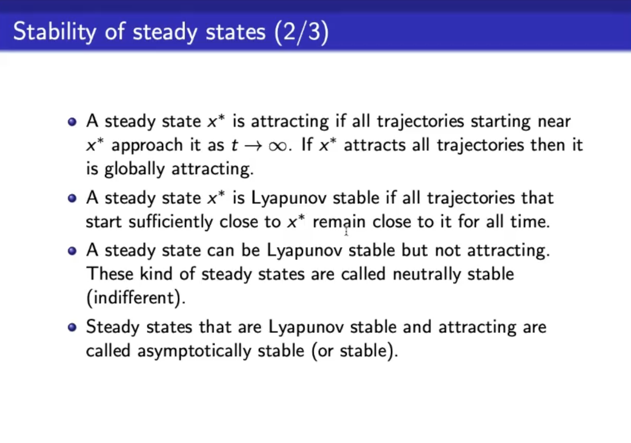
• Definition of “attractive ss”, “Lyapunov stable ss”, “neutral ss” and “asymptotically stable ss”
  • We have seen “Lyapunov stable ss” previosly for the oscillating pendulum, without friction* (blac circular lines in the phase space).

• marginally stable ss are an example of Lyapunov stablity
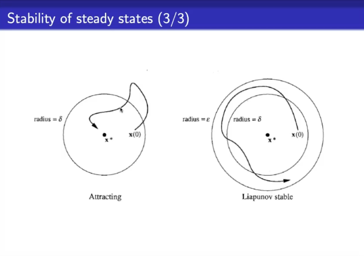
• for asymptotic stability we need to say that the flow will always get closer to the ss, notice how in this example for attracting ss the flow first moves away the ss

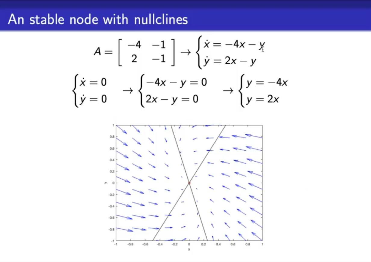
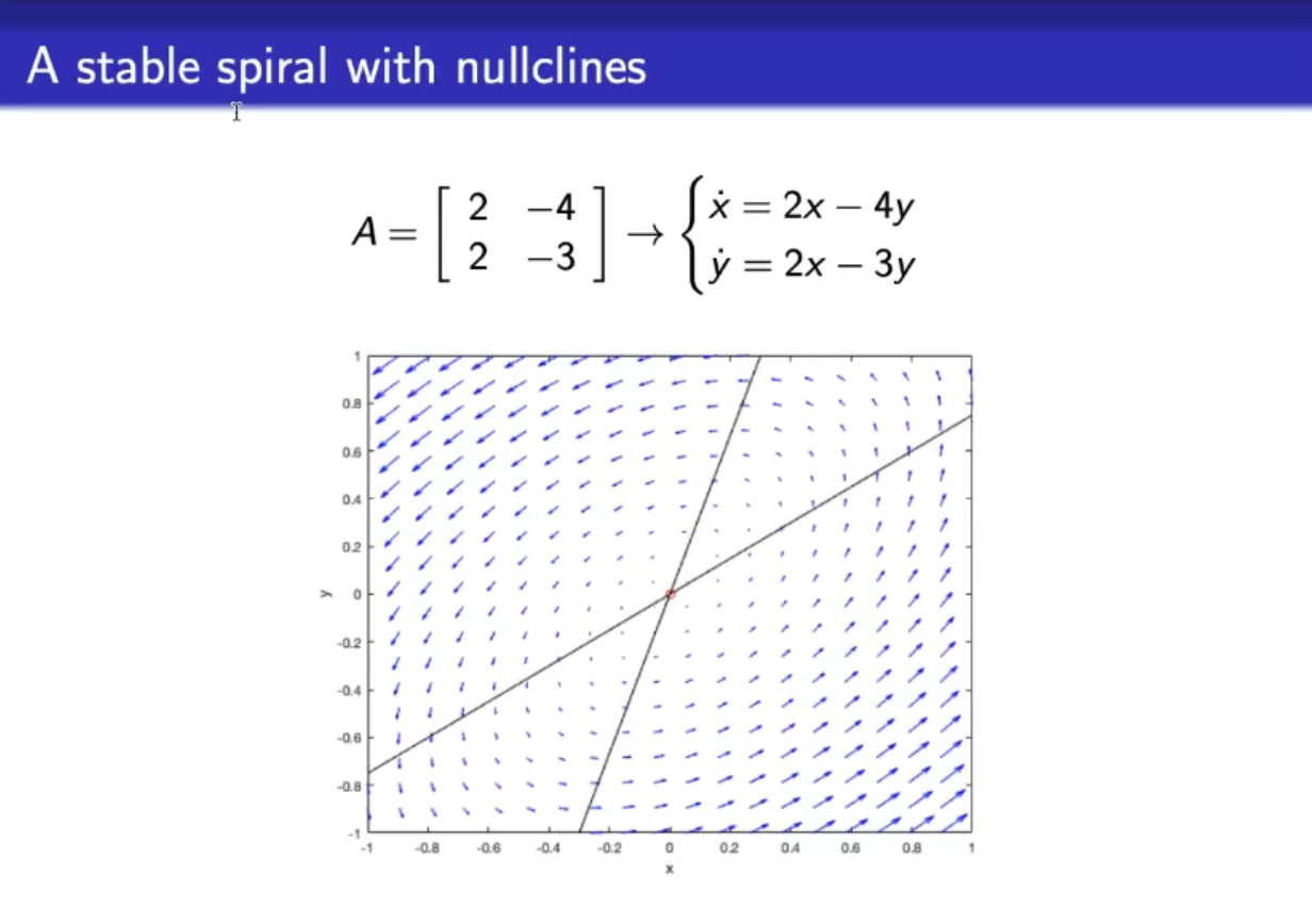
• The nullclines are in this case:
  • $y=-4x$
  • $y=2x$
  • And are represented in the phase space as the black lines.
• The blue arrows are found via a simulation.
• This should be an attractive ssnot-sure-about-this

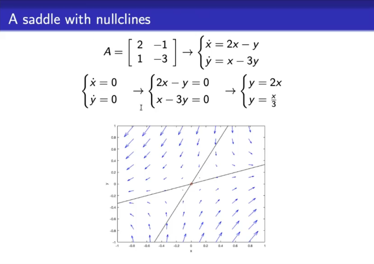
• The $(0,0)$ point this time is an unstable ss.

• asymptotically stable ss
• Negative eigenvalues, we will see more in detail later

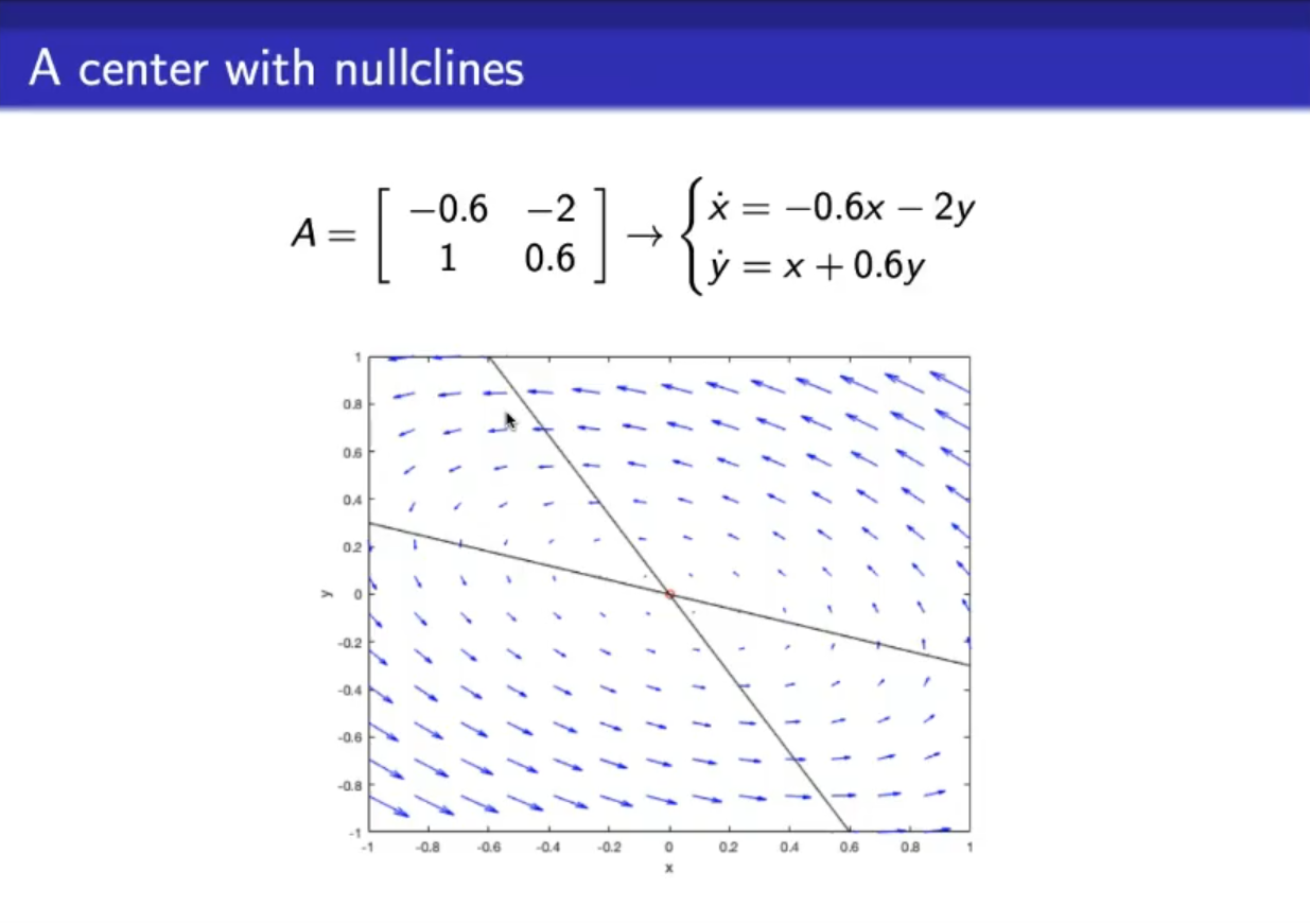
• Lyapunov stable ss
• Immaginary eigenvalues, we will see more in detail later

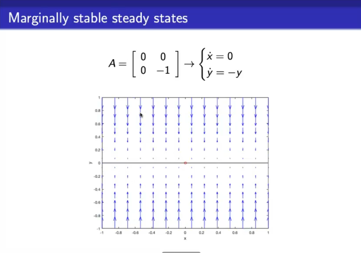
• marginally stable ss

---

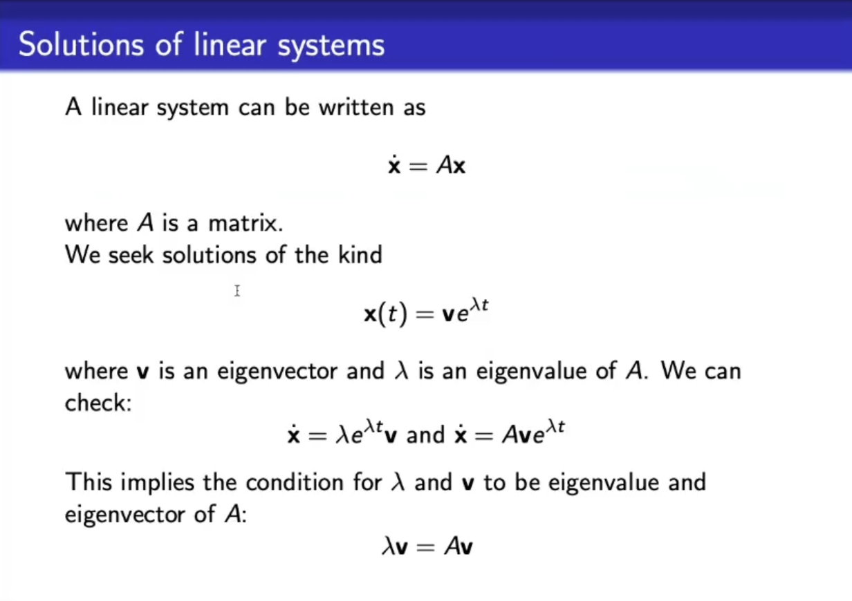
• For each system that does not include a constant, so for $\dot{x}=Ax+c$ where $c=0$, then $x=0$ will always be a ss.

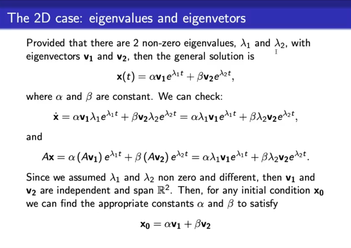
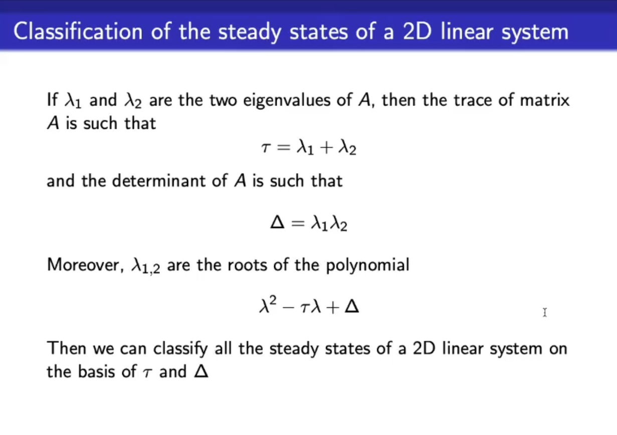
• Example of an explicit analitic solution for a 2D general case,NOT-IMPORTANT

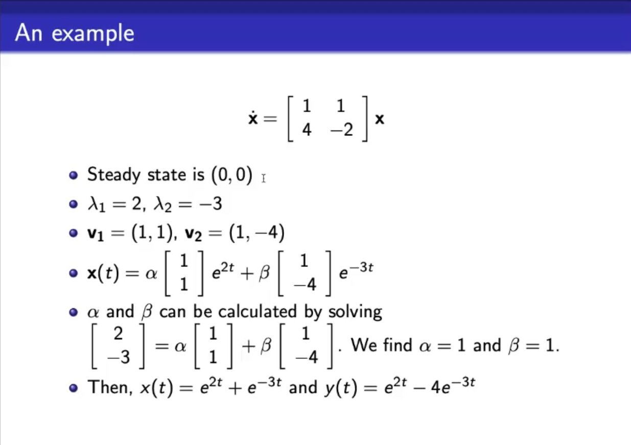
• Basically we have found a general solution for 2D linear systems in the form $\dot{x}=Ax$, but this is just an example, we will solve systems numerically and not analitically.

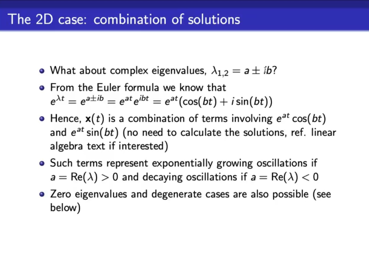
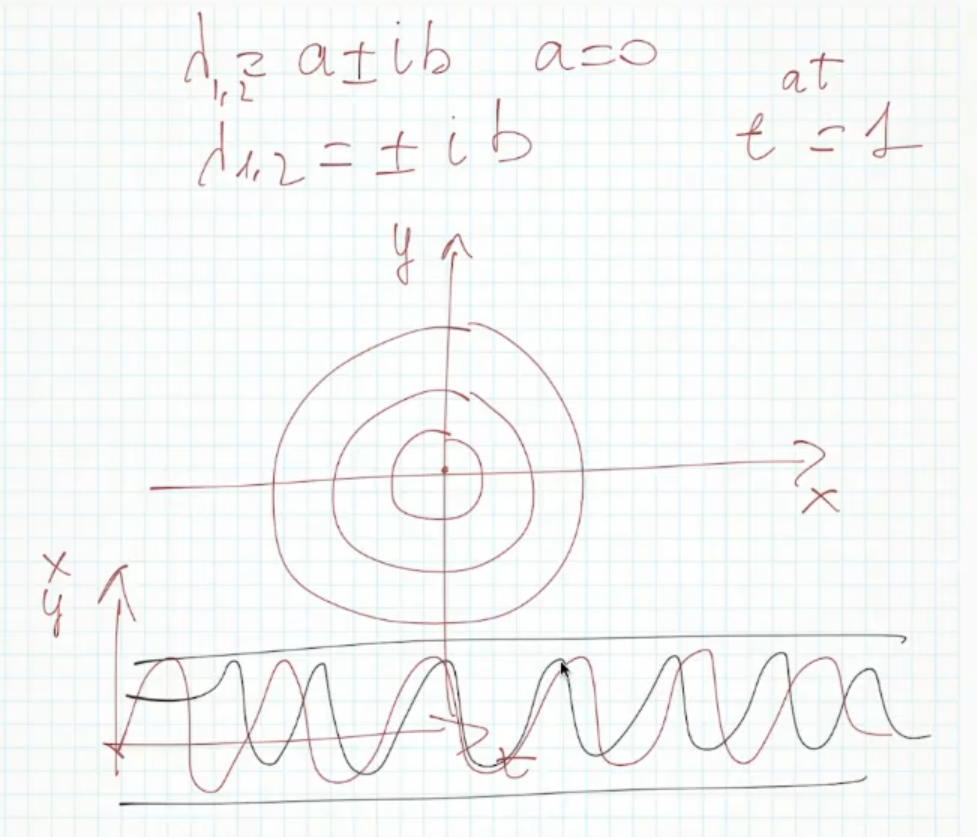
• In case we deal with complex eigenvalues.
• However, again, we will not use this.not-sure-about-this
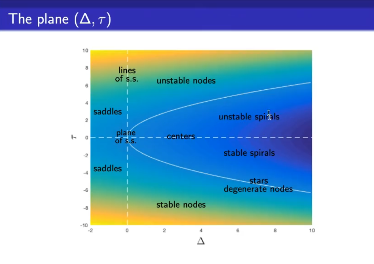
• It is important to understand the difference between positive/negative and real/complex eigenvalues.IMPORTANT

Let’s make an example: where we take 2 negative eigenvalues 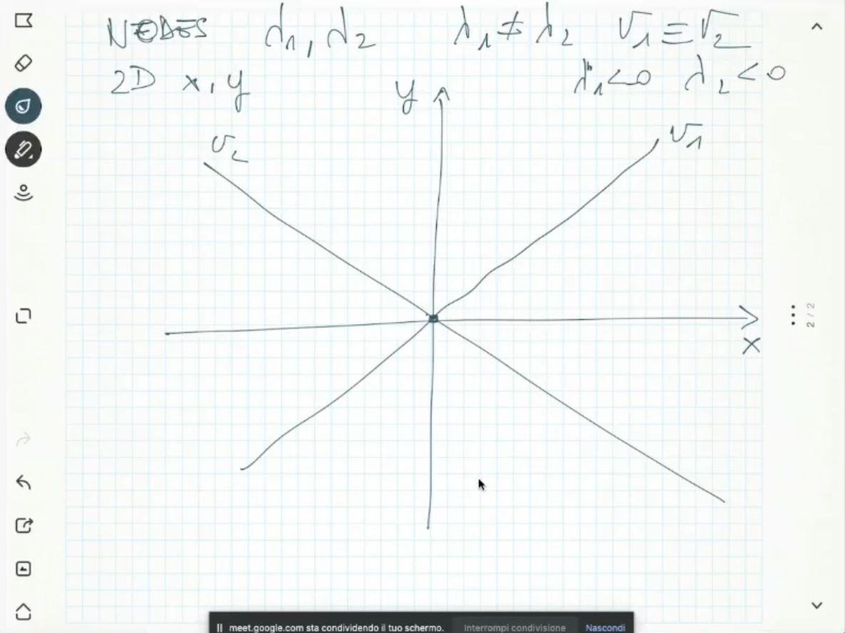${\lambda }_1$ and ${\lambda }_2$:

We can draw the flow, suppose 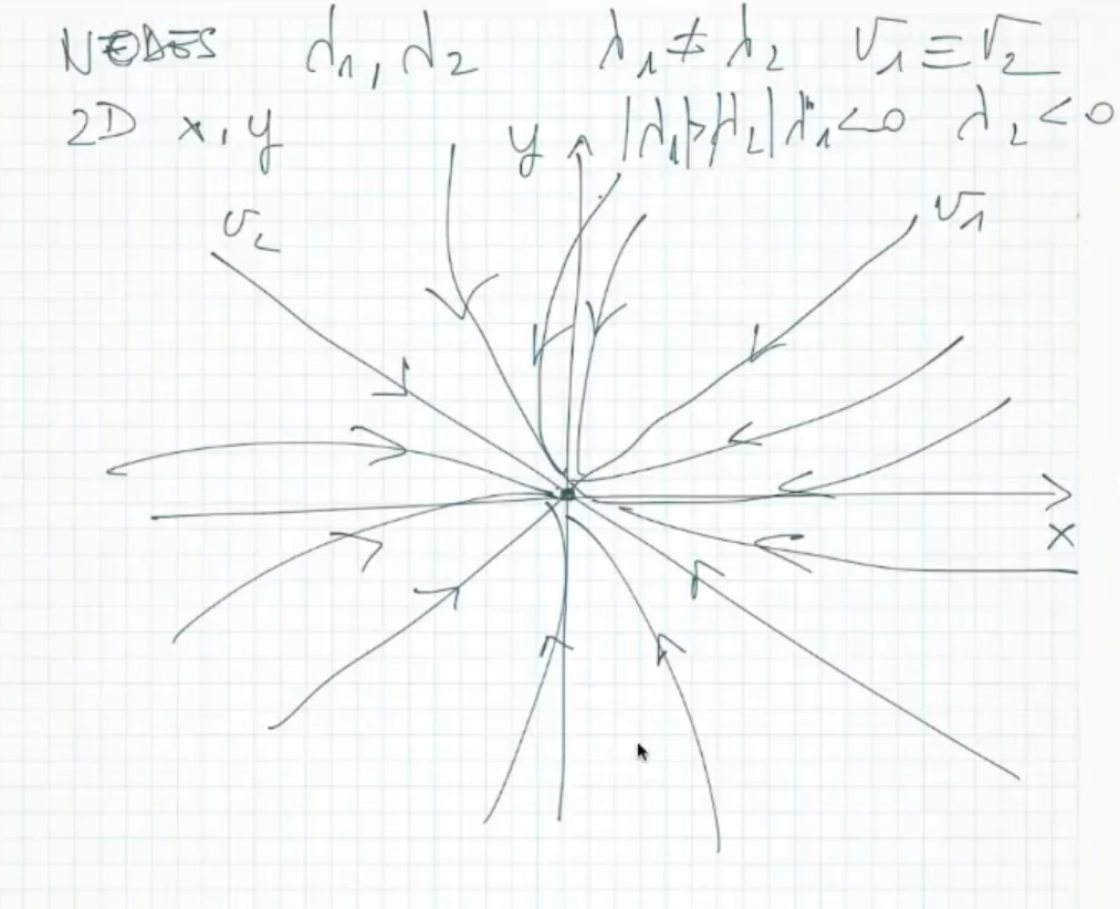$|{\lambda }_1|>|{\lambda }_2|$:

Also if instead we took the two eigenvalues both positives, the geometry would have been the same, but the flow would have been reversed (unstable ss):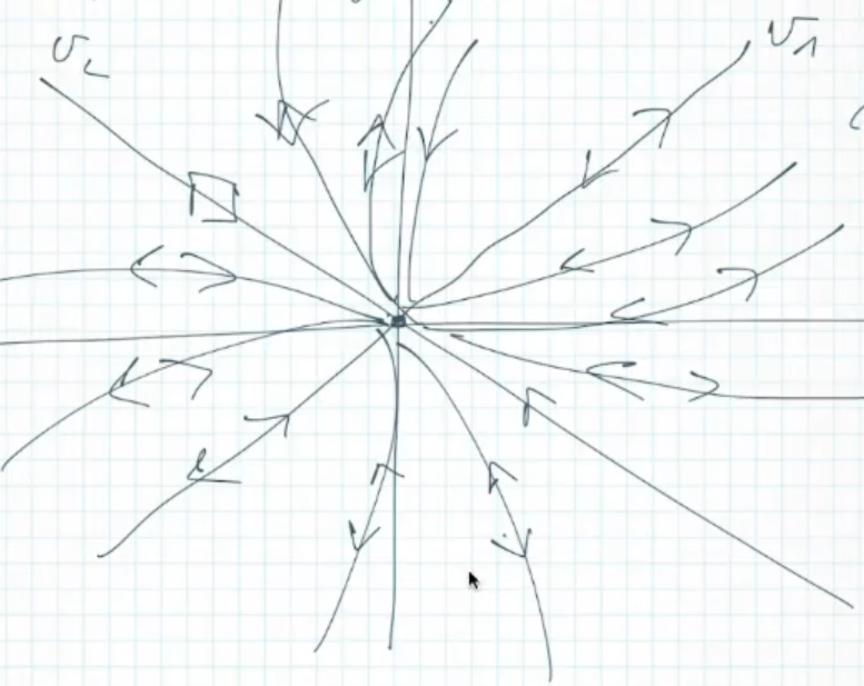

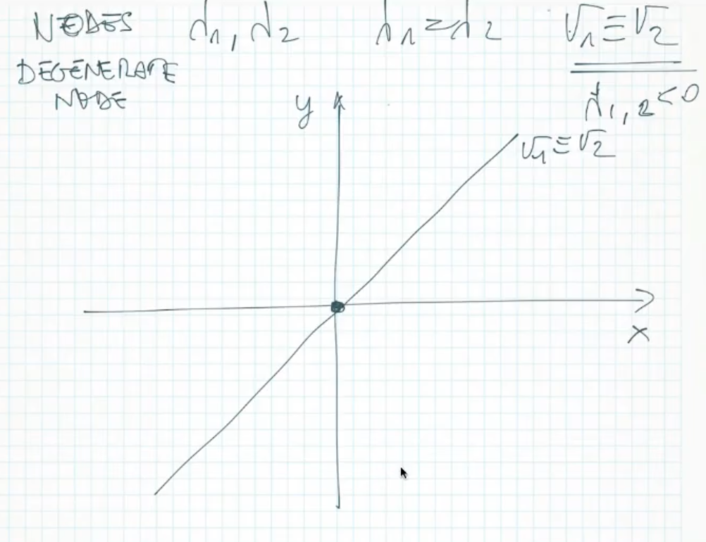
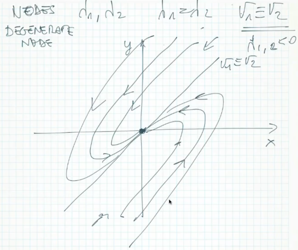
Example of “degenerate node”, with both ${\lambda }_1<0$ and ${\lambda }_2<0$, and $v_1=v_2$:

Again if we change: ${\lambda }_1>0$ and ${\lambda }_2>0$, we obtain the same geometry with inverted flow: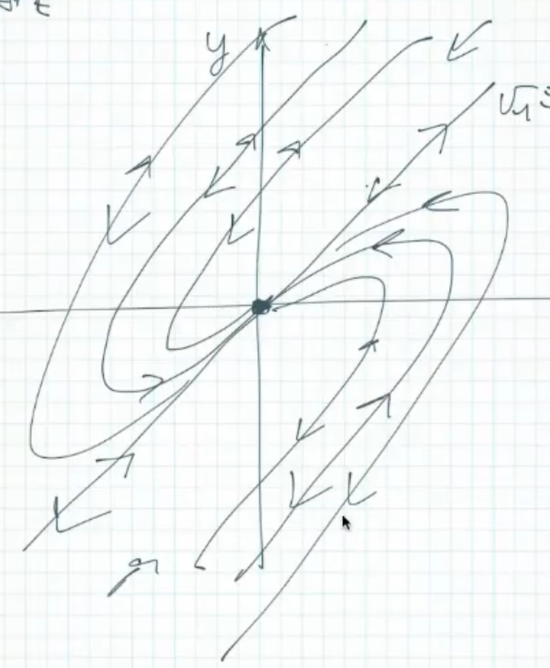

• We can say that degenerate nodes lie in-between nodes and spiral.

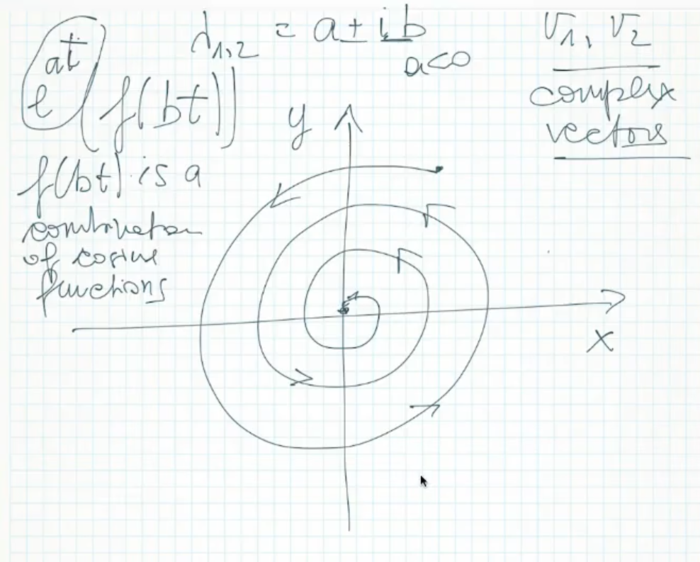
Complex eigenvalues: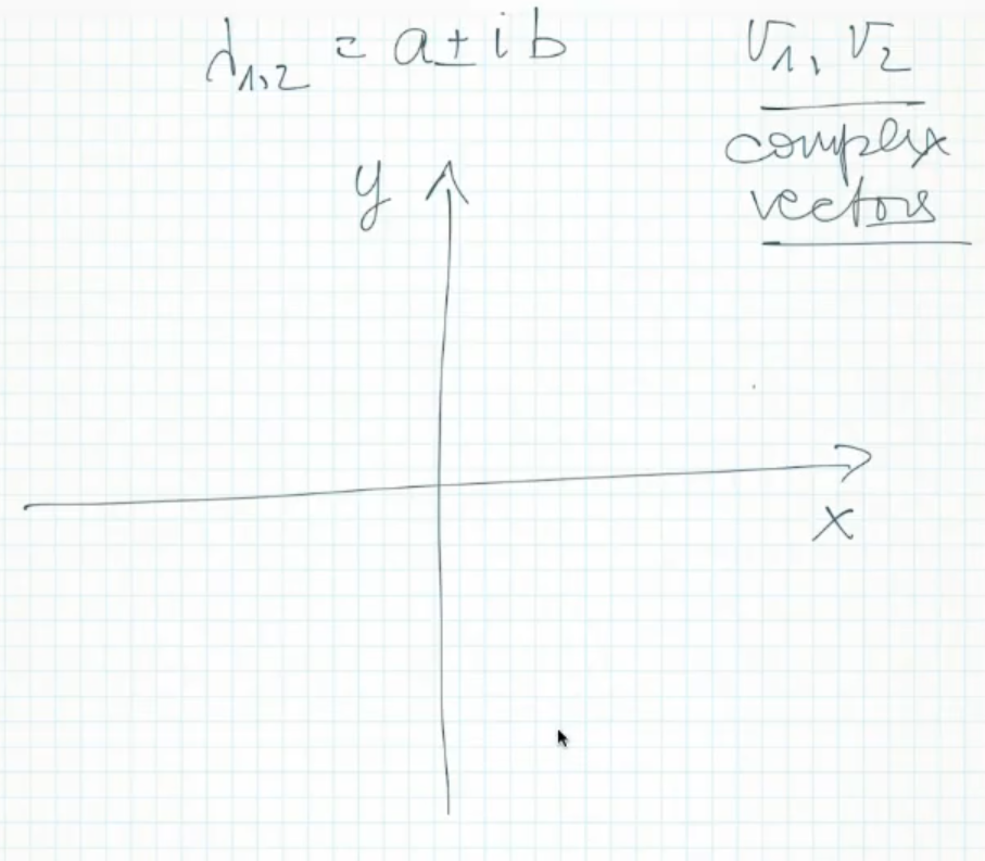

• For $a<0$:
  
• Remeber that if we where to draw the evolution of $x$ over $t$ (the “dynamics graph”) we would have:
  
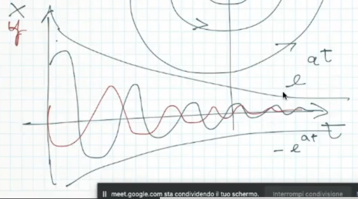
• Like before for $a<0$ we would invert the flow.
• For $a=0$: