CDS - Syncronization for Dynamical Systems on Graphs • Attributes of Graphs and Networks

Remember:

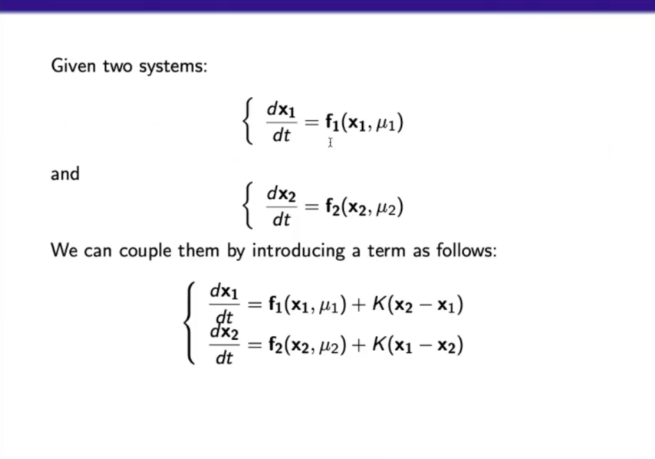
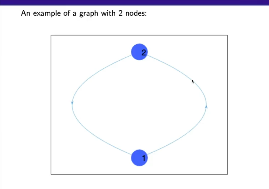
We can represent the “coupling” of multiple systems with a connected graph:

Where each node is a system.

REMEMBER: A graph is a mathematical object defined by a given number of nodes and a given number of links connecting the nodes
A graph has many properties, it can be directed or undirected, in this case the graph is directed, since there is a “direction of influence” (the links have arrows).
We will se also other properties.

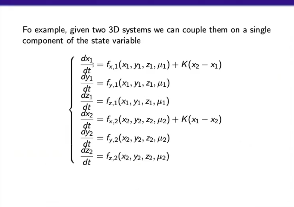
We can see the effect of syncronization, by taking 2 Lorenz systems, and adding a coupling term, such that only the variable $x_{1}$ of the two system is connected to each other: $k (x_{1}^{'} - x_{1}^{''})$ and $k (x_{1}^{''} - x_{1}^{'})$ , since only one variable is coupled we defined this as a “weak coupling”. Also we consider the Lorenz systems in the chaotic regime, so for $r > r_{H}$ , and we also take two initial conditions really near each other, so to show the sensitivity to initial conditions.

Base example with $k = 0$ (no coupling):

$k = 1$ :

$k = 10$ :

For $k = 10$ we have much more similar systems ⇒ the two systems are syncronized.

Some type of graphs and examples:

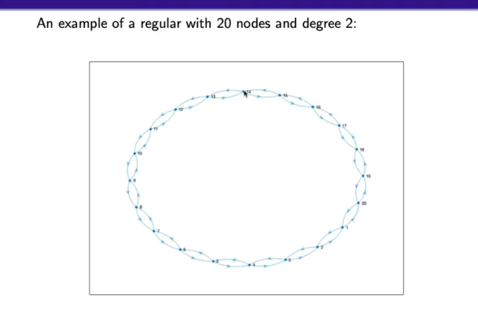
Regular ring network of degree 2:

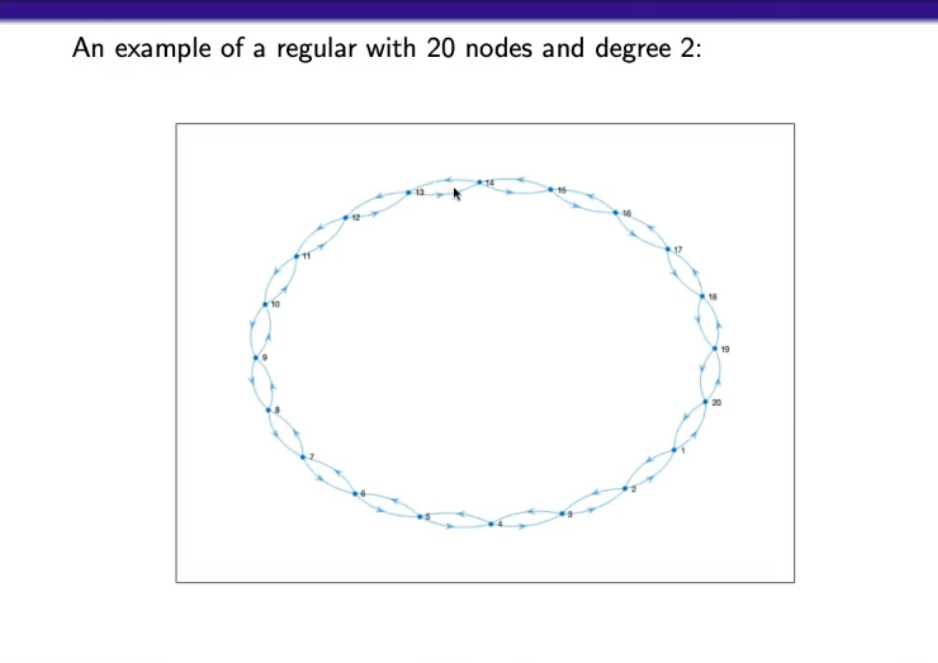
This is called a “ring network”.

This particular case has bidirectional connections.

And has degree 2 because each node is connected to 2 nodes.

Regular ring network of degree 4:

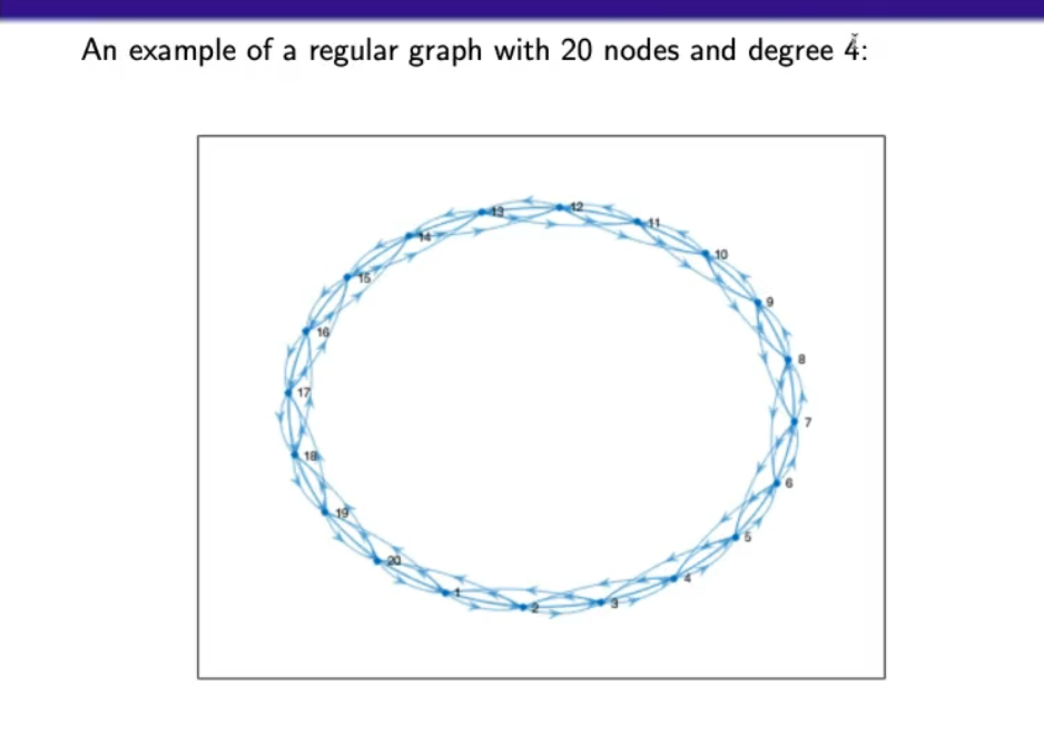
Degree 4: each node is connected to 4 nodes.

Erdos-Renyi graph of degree 2:

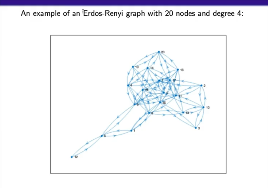
Erdos-Renyi graph of degree 4:

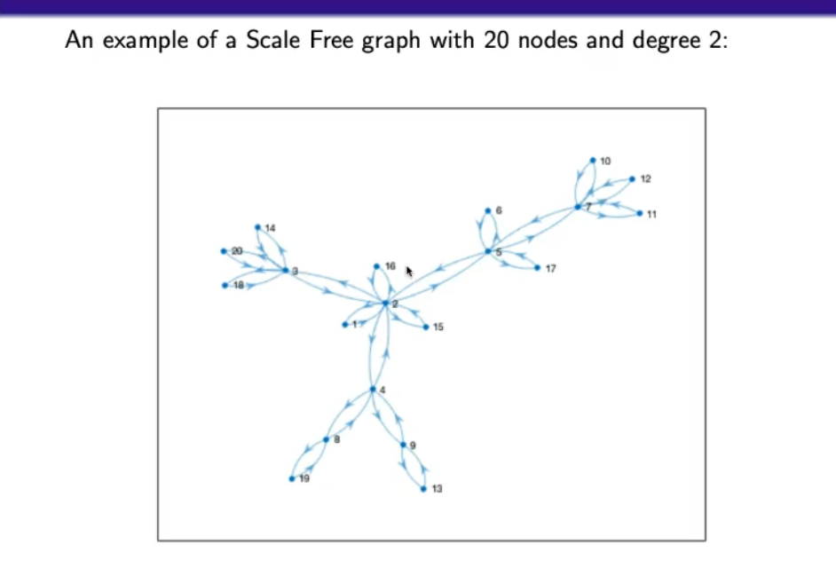
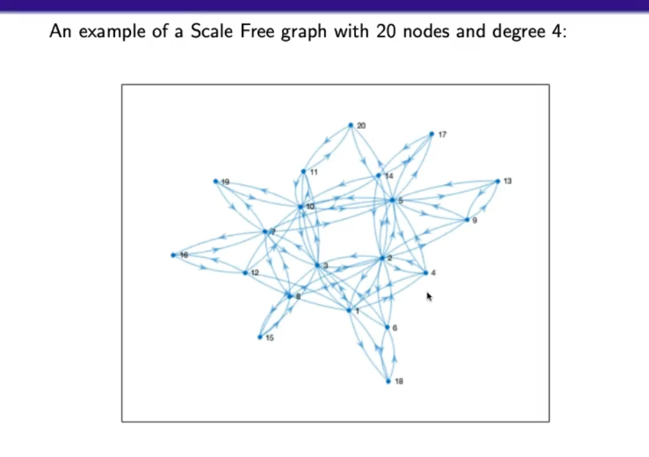
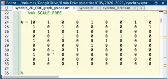
Scale-Free graph of degree 4:

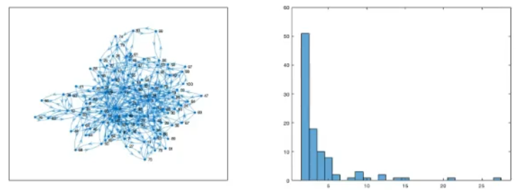
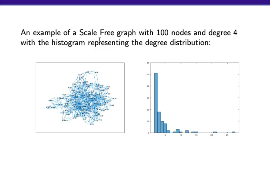
Scale-Free graph with 100 nodes and degree 4, with histogram represengin the degree distribution:

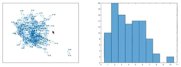
Erdos-Renyi graph with 100 nodes and degree 4, with histogram represengin the degree distribution:

To summarize:

A regular graph has vertices all with the same degree

A graph of degree $n$ is typically understood as an $n$ -regular graph.

An $n$ -regular graph is a regular graph where each vertex has a degree of $n$ , so it is a repetition of graph of degree $n$ .

An Erdős–Rényi graph is a type of random graph, introduced by Paul Erdős and Alfréd Rényi. It is one of the simplest and most studied models of random graphs. There are two closely related definitions of an Erdős–Rényi graph:

In the $G (n, p)$ model, an Erdős–Rényi graph is defined as follows:

$n$ : the number of vertices in the graph.

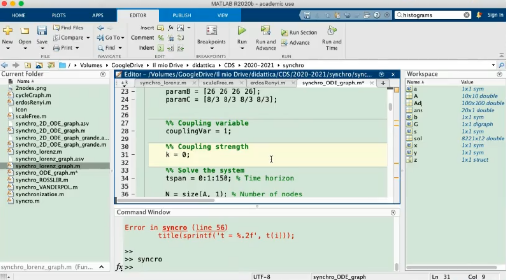
$p$ : the probability that any given pair of vertices is connected by an edge.

In the $G (n, M)$ model, an Erdős–Rényi graph is defined as follows:

$n$ : the number of vertices in the graph.

$M$ : the number of edges in the graph.

A scale-free graph is another type of random graph characterized by a power-law degree distribution. This means that the number of vertices $k$ with a degree $d$ (the number of connections or edges) follows an arbitrary distribution $P$ .

The ending part of the graph are called “leaf”, they are connected to only one other node.

Also we have talked about “hubs”, which in the context of network theory and graph theory is a vertex (or node) with a significantly higher degree compared to other vertices in the graph.

These graphs can all be considered “undirected”, meaning that each connection has a “counterpart”
~Ex.: Node 4 is connected to node 5, but node 5 is also connected to node 4, this is true for all nodes.
More precisely: “a graph is defined as undirected if the “matrix structure” $A$ , is symmetric”.
Also an undirected graph has always same number of in and out degree for each node.

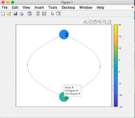
The In Degree (number of “arriving” connections)

The Out Degree (number of “exiting” connections)

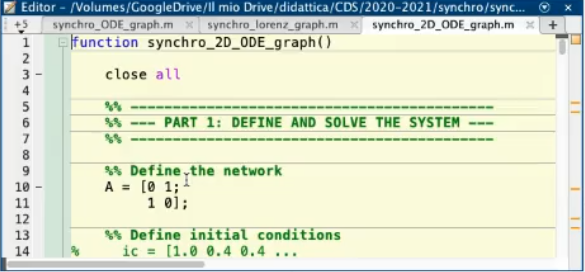
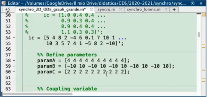
Let’s take ten systems, in a regular ring network, and we define their connections via the $A$ matrix:
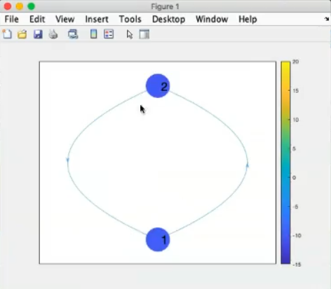
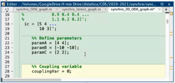
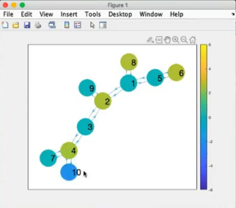
This is the graphical view of the graph:
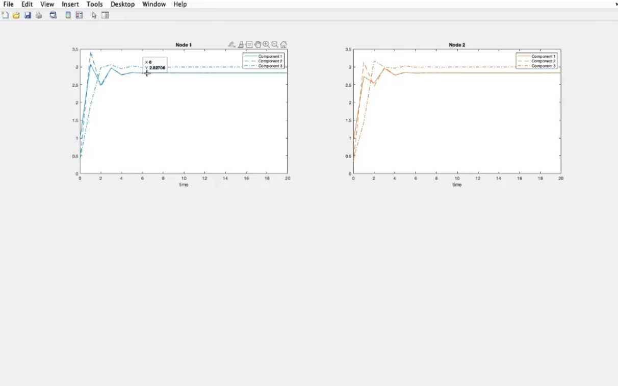
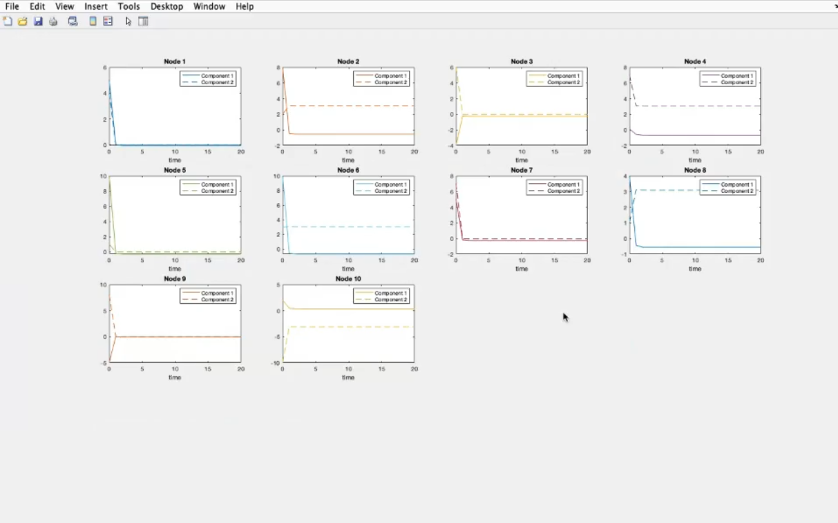
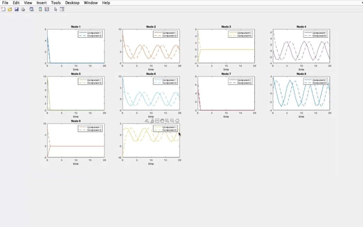
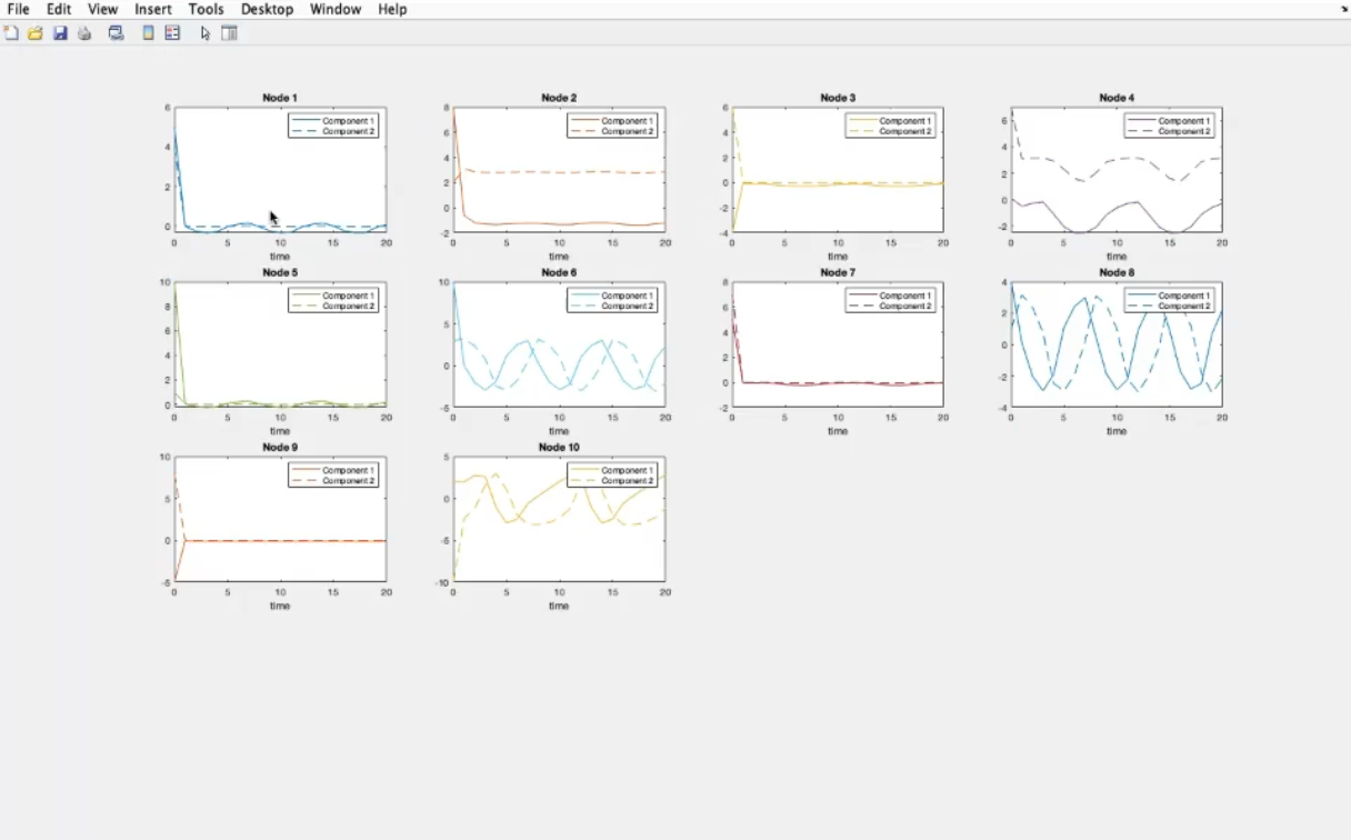
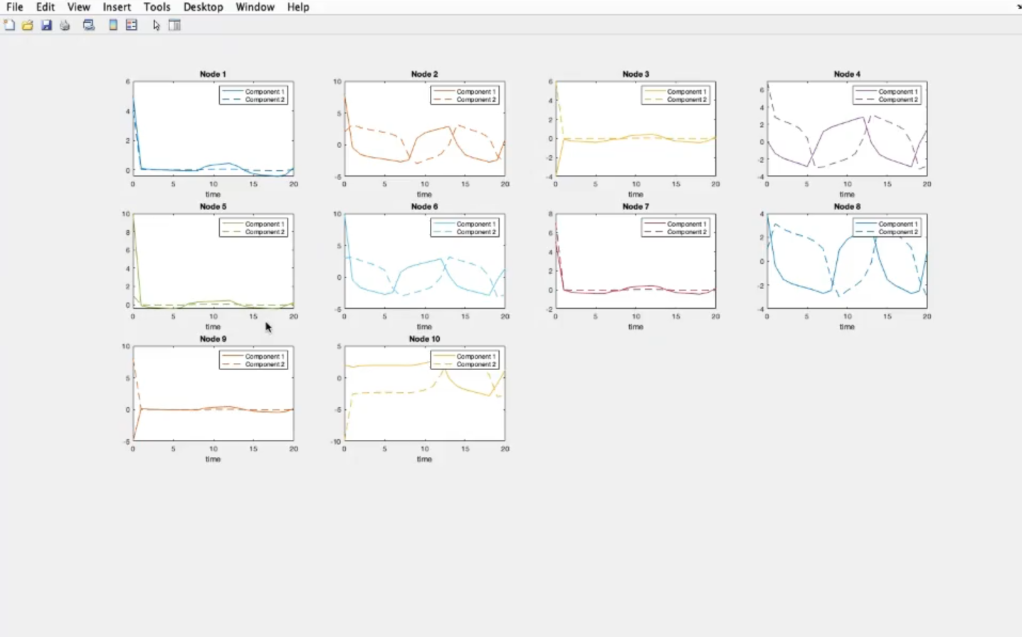
After defining the systems, draw a system-wise graphs: Each graph corresponds to a system, an in it there are represented its component changing with time $t$ . This is the case without coupling, so for $k = 0$ . These are 10 systems each with 2 components, in these system there are some oscillating ones, and a few of them instead converge at a specific value. Also only the first component is coupled. Now let’s see how the system changes:

For $k = 4$ :
The majority of them should oscillate, but as we can see the converging node help the network stabilize.

For $k = 1$ :
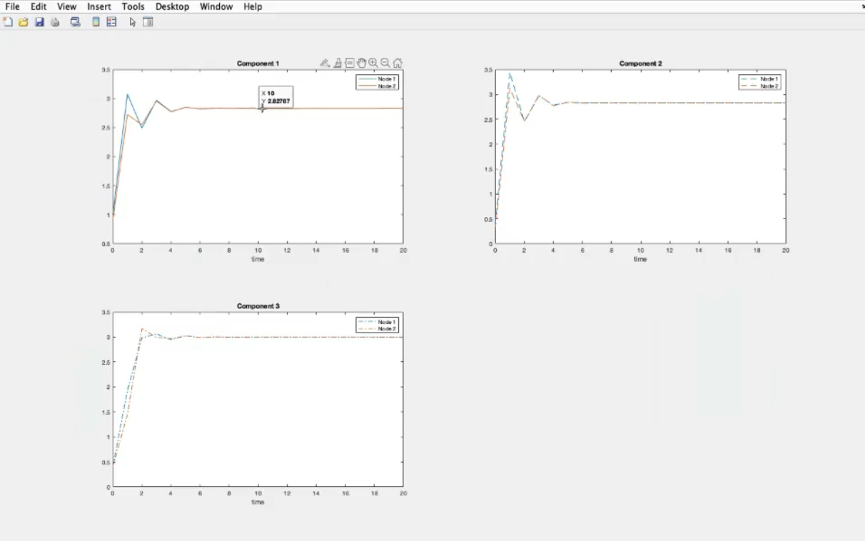
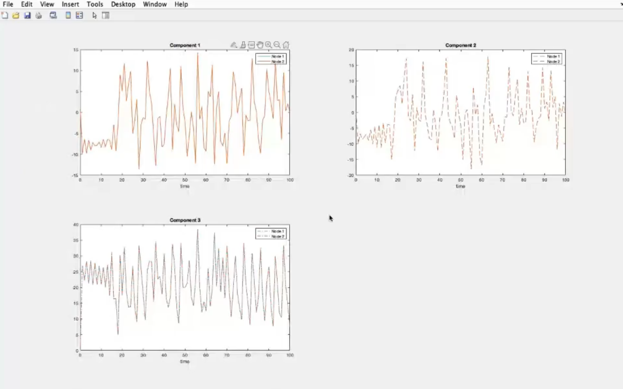
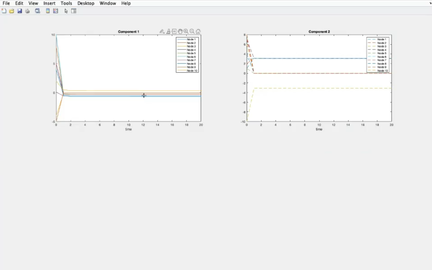
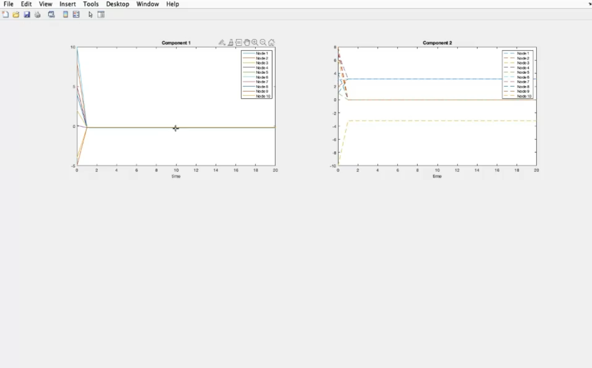
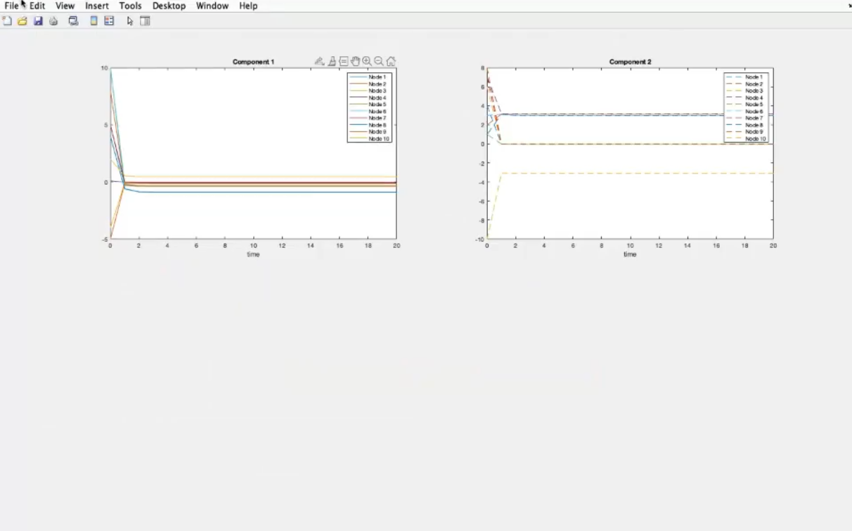
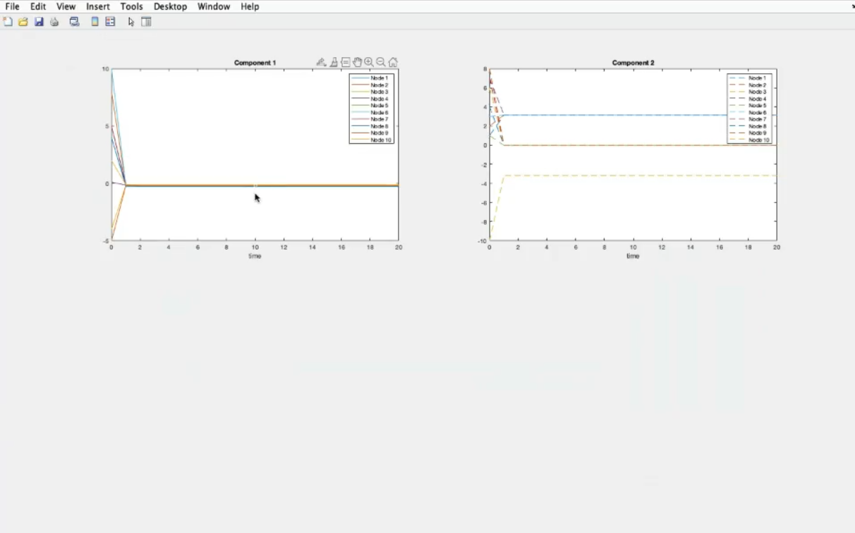
They influence each other, but there is no “dominating system”.

For $k = 100$ (component-wise graphs: each graph represent a different component, remember that these are 10 system each with 2 components):
As you can see the first components (the coupled component) all converge at the same value, while the second components (which are not directly coupled do reach convergence as well, but not at the same value)

Same 10 systems as before but with different graph/network-strucutre, scale free graph:

For $k = 0$ (system-wise plot):

For $k = 1$ (system-wise plot):

For $k = 6$ (component-wise plot) as you can see the systems are syncronized:

For $k = 100$ (component-wise plot) as you can see the systems are stabilized:

NOTE: In this case the shape of the network does not change much about stability or syncronization, but (in general) it absolutely can.

Graphical representation of the connection.
Each node is a system.
REMEMBER: A graph is a mathematical object defined by a given number of nodes and a given number of links connecting the nodes
A graph has many properties, it can be directed or undirected, in this case the graph is directed, since there is a “direction of influence” (the links have arrows).
We will se also other properties.

Now immagine that the simple 2-node graph seen previusly describes two Lorenz systems, connected.
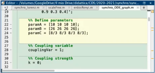
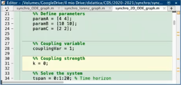
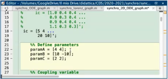
Also consider a “weak coupling”, such that only the variable $x_{1}$ of the two system is connected to each other: $k (x_{1}^{'} - x_{1}^{''})$ and $k (x_{1}^{''} - x_{1}^{'})$ .
Base example with $k = 0$ (so we are in the case of no-connection / independent systems), and these are the intial conditions and parameters of the two systems:
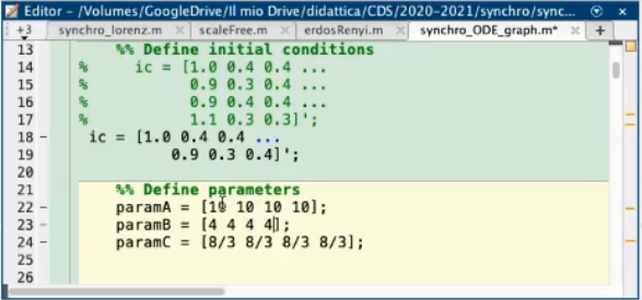
- paramB: is what we define as $γ$ .
- paramC: is what we define as $β$ .

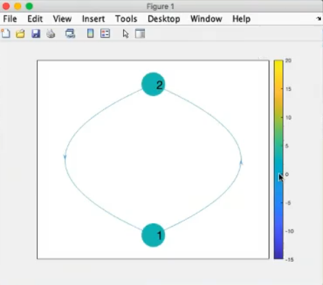
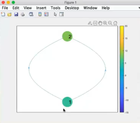
The color represents the value, it does not change much and it remains near $0$ .
It is more or less stable.

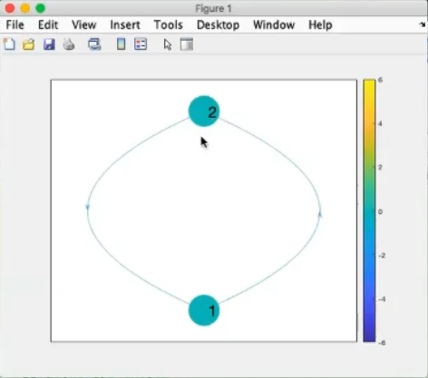
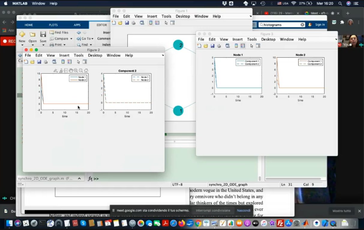
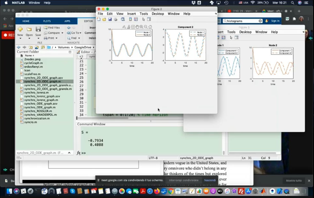
After solving the system, this are the results, since the system is stable, both system convergee to the same results.
We hare in the case of “after the pitchfork bifurcation” of the Lorenz system.

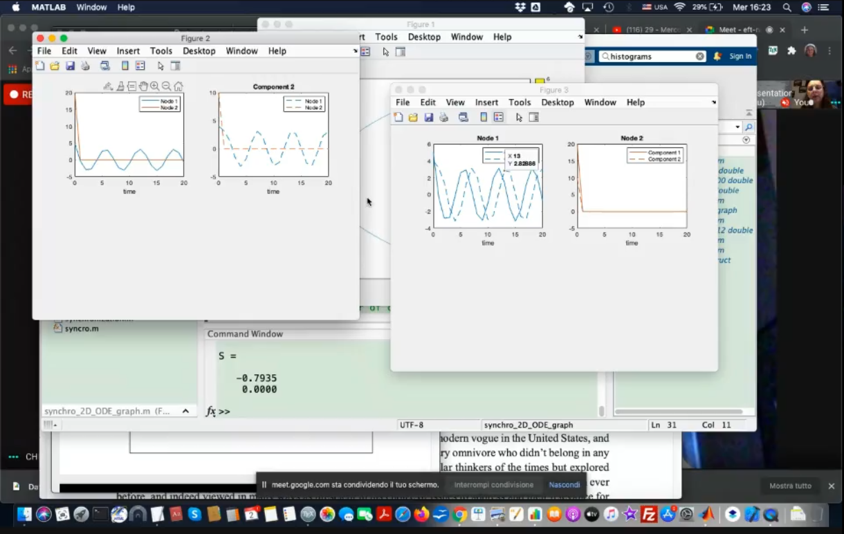
Here we see the same graphs as before, but divided into the two systems, as you can see the only difference is the transients.
REMEMBER: We are in the case of indipendent systmes, they converge to the same results because they have the same parameters and are “converging systems”.

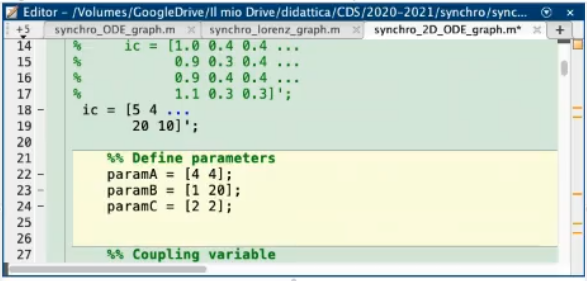
We now move the system into the chaotic regime, by changing paramB.
Still $k = 0$ ⇒ indipendent systems.

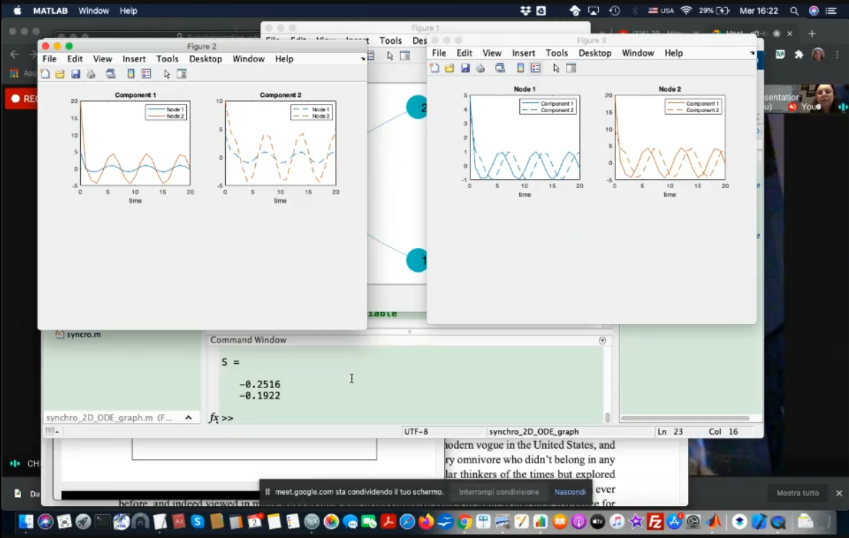
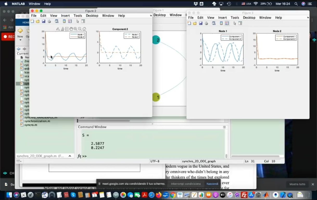
The node now change colors frequently, and can assume different colors at the same time, here’s another shot:

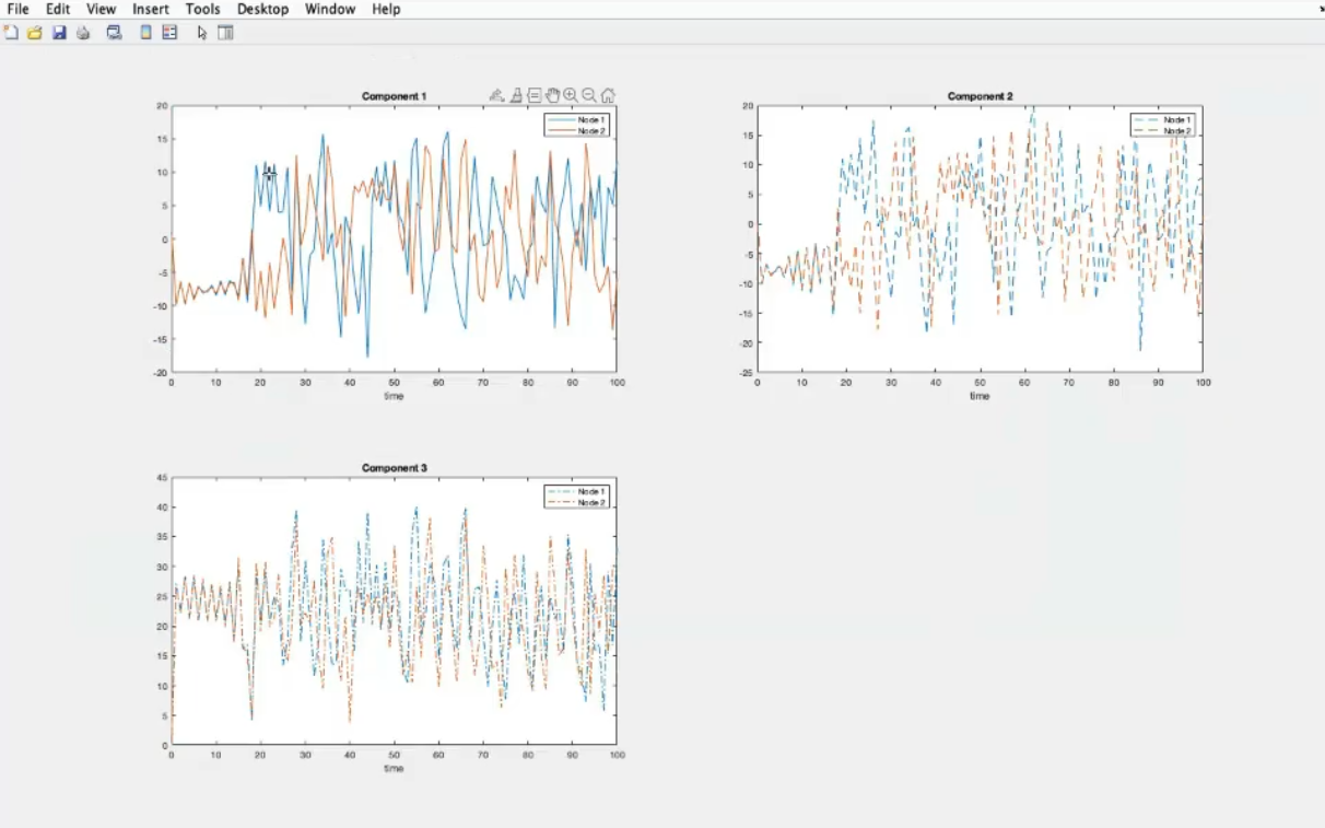
Division in components, you can see the chaos.

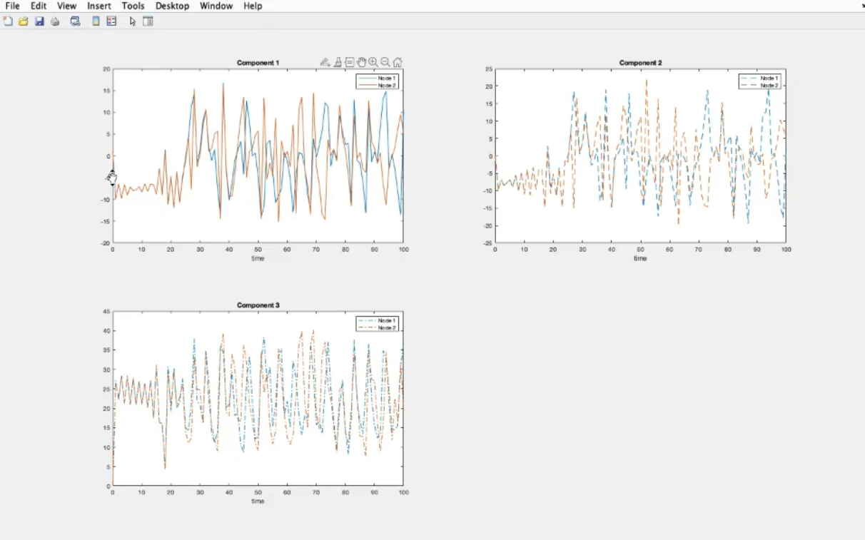
$k = 1$ , results are almosts the same as before.

$k = 10$ , much more similar systems ⇒ the two systems are syncronized.
So we have seen that chaotic system can syncronize.

Bidirectional connections.
This is called a “ring network”.

degree 4: each node is connected to 4 nodes.

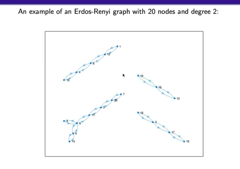
Erdos-Renyi: random graph, in this case degree 2 refers to a medium of connections.

The 12° node is called a “leaf” (it has very few connections)

There is only 1 graph (we can always find a list of connections from one node to another)
We can define some hubs like node 2, 3, 4, 5, 7.

Still some hubs and leaves.

Many leaves (nodes with little connections).
Few higher degree nodes, from the picture we can define the hubs.

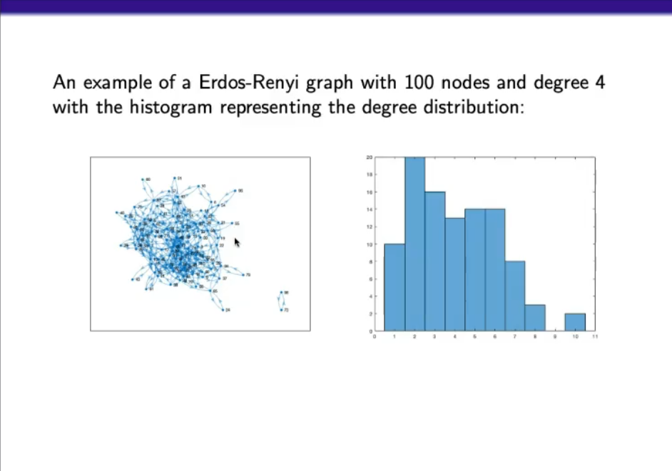
There can be separation (not all nodes can reach all the others)
The maximum degree is lower thatn that of the “Scale Free graph”.

Each node represents a dynamical system.
We will see how different type of graph handle changes, how the change of a node can spread, and the syncronization.

Simplest graph with only 2 nodes.

2 Identical stable systems, with different inital conditions, and NO coupling.

Graph

Changing paramB, the systems will now oscillate.

The two system are slightly different, due to the different inital conditions

Changing paramB, this time the systems are diffrent.

One oscillating and one converging system

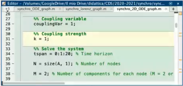
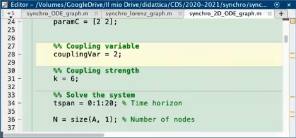
We now introduce coupling: $k = 1$ . (pretty weak)

We can see some effects, but since $k$ is small, not very much.

$k = 6$
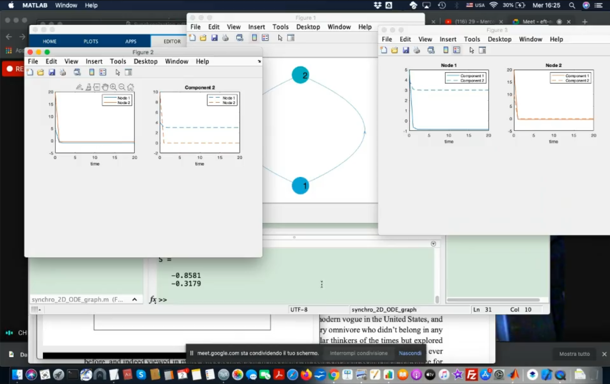
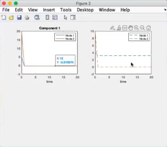
Now both system converge, however the 2nd components converge to different values, specifically to $- 1$ and the other to $3$ .
The 1st component of both systems converge almost to the same value, since these are the coupled components.

We switch coplingVar from 1 >> 2, meaning that now the coupled components are the 2nd ones.

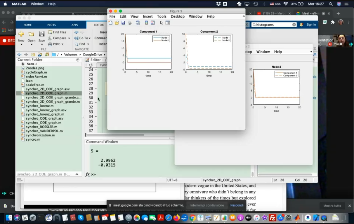
$k = 60$ , the 1st components coincide at regime, the 2nds are still different.

Regular large network, each node still represents a hopf bifurcation.
Some node have negative $θ$ some have a positive one.

Graph

$k = 4$
The majority of them should oscillate, but as we can see the converging node help the network stabilize.

$k = 0$ (indipendente nodes)

$k = 1$
They influence each other, but there is no “dominating system”.

$k = 100$
The system is stabilized.

Now we change the shape of the network/graph.

Graph

$k = 0$

$k = 1$

$k = 6$
The system is syncronized.

$k = 100$
The system is stabilized.
NOTE: In this case the shape of the network does not change much about stability or syncronization, but (in general) it absolutely can.

🪴 Quartz 4.0

Explorer

CDS - Syncronization for Dynamical Systems on Graphs • Attributes of Graphs and Networks

Remember:

Graph View

Backlinks