CDS - Lecture 6

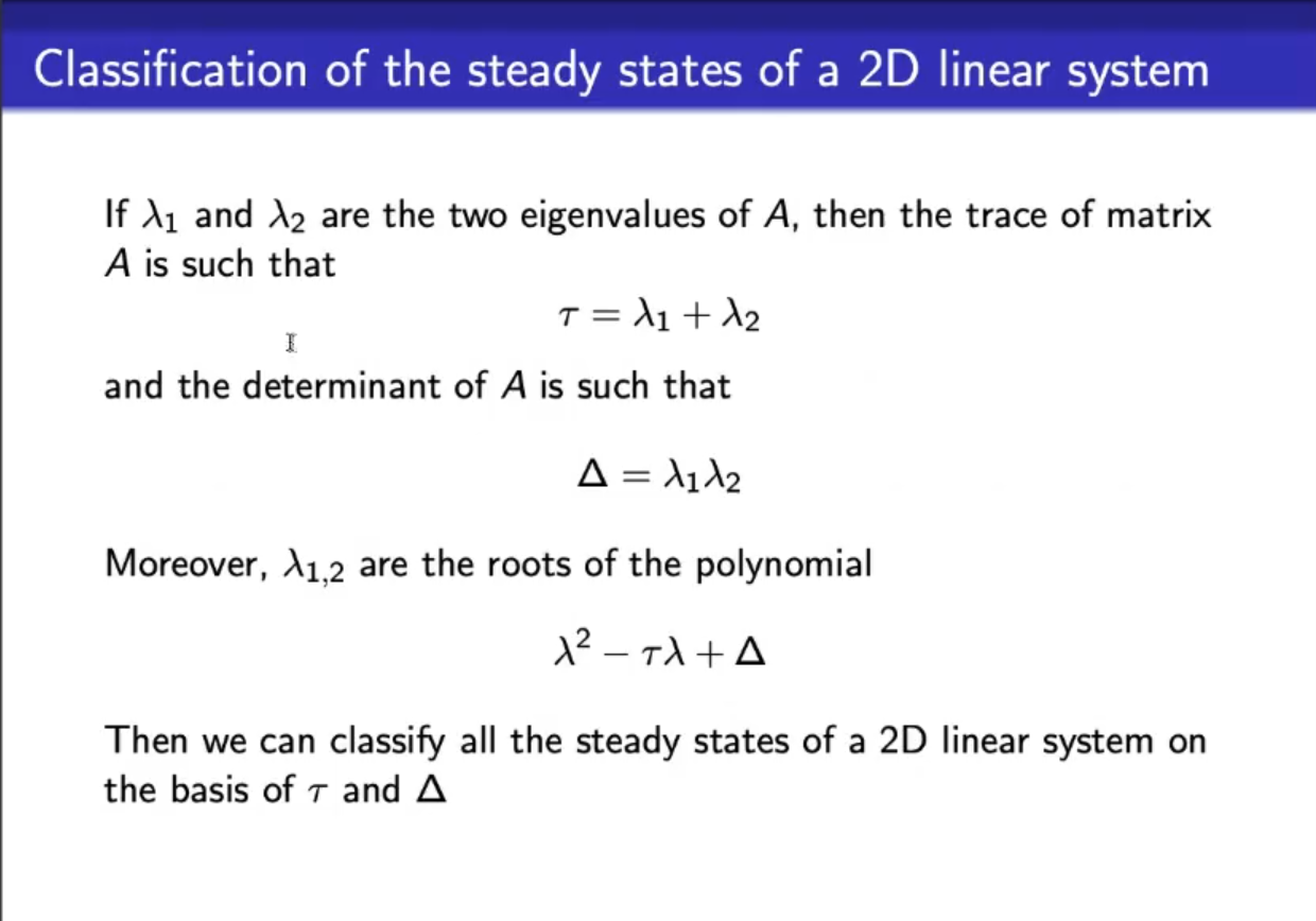
• ${\lambda }^2-\tau \lambda +\Delta$ is called the “charateristic polyomial”

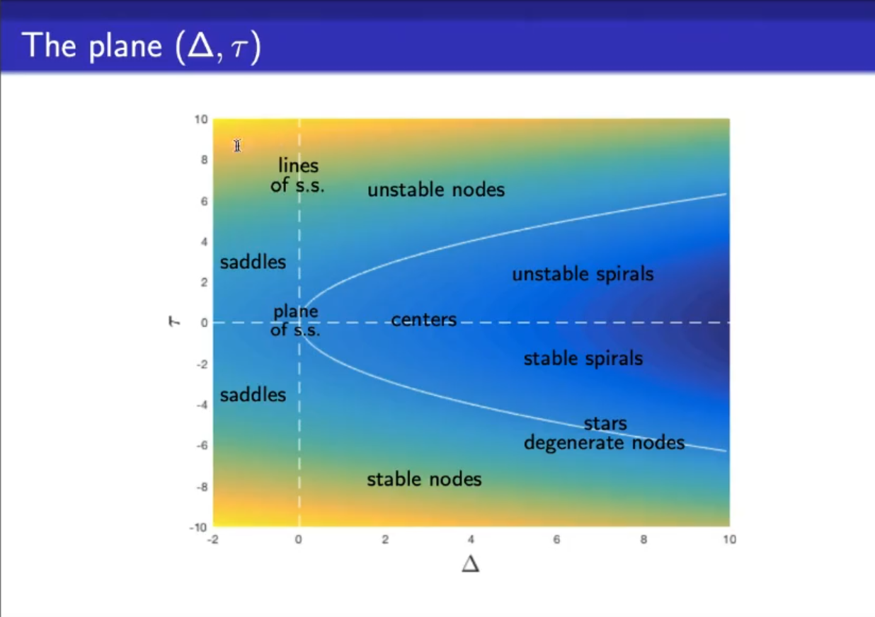
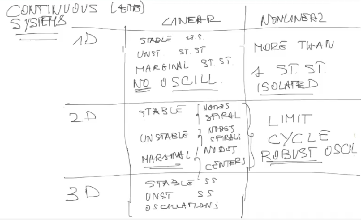
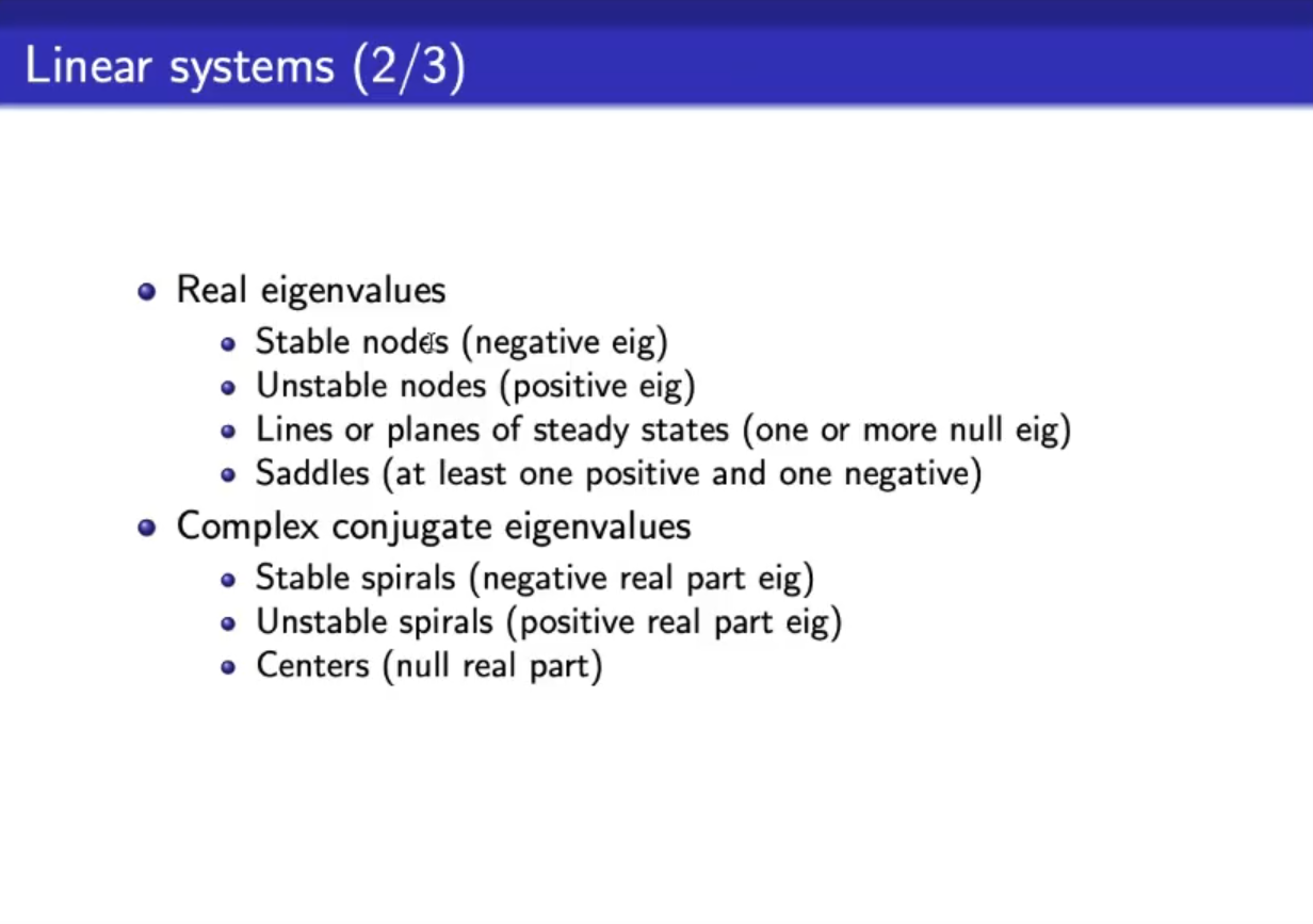
• This is the plot, and with this we can define all the “types of nodes” or flow, for a 2 dimensional system.
• Remember that:
  • $\tau ={\lambda }_1+{\lambda }_2$
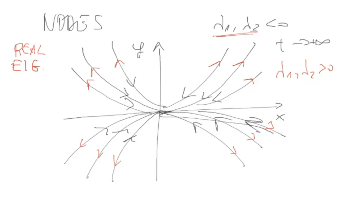
  • $\Delta ={\lambda }_1\cdot {\lambda }_2$ Example of nodes (stable - black flow, and unstable - red flow):
    

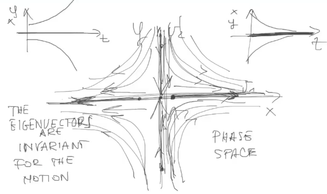
Example of a saddle: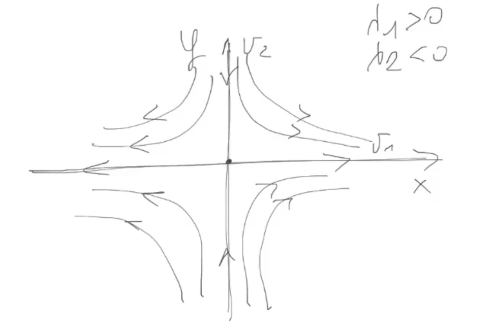

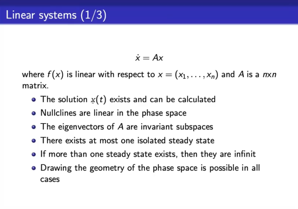
Analizing the initial conditions on the $x$ and the initial conditions on the $y$ axis, we have made example also in the dynamics graph, and said that: The eigenvectors are invariant for the motion.

• However this is not very clear/useful i think (Lecture 6 27:00)not-sure-about-this

Stable (in red) and unstable (in black) spiral: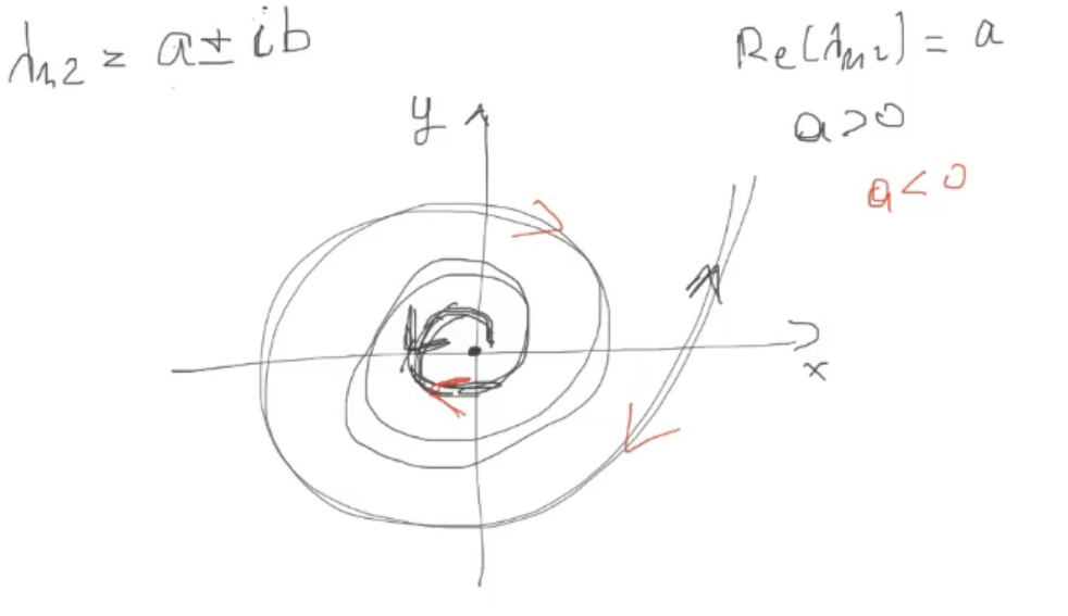

• The dynamics, stable spiral:
  
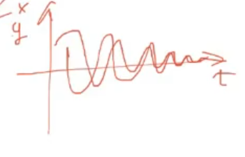
• unstable spiral:
  

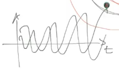
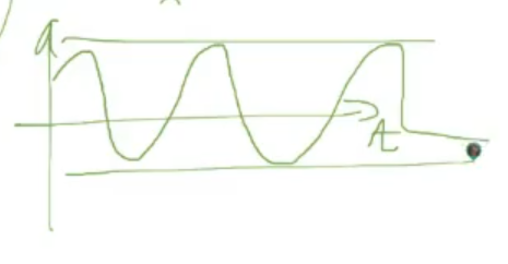
While in case of “centers” (for 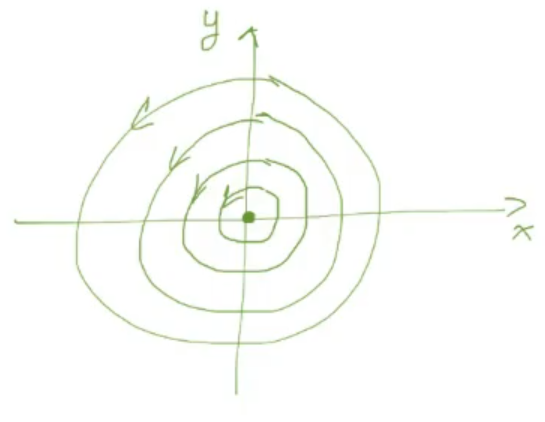$a=0$):

• The dynamics:
  

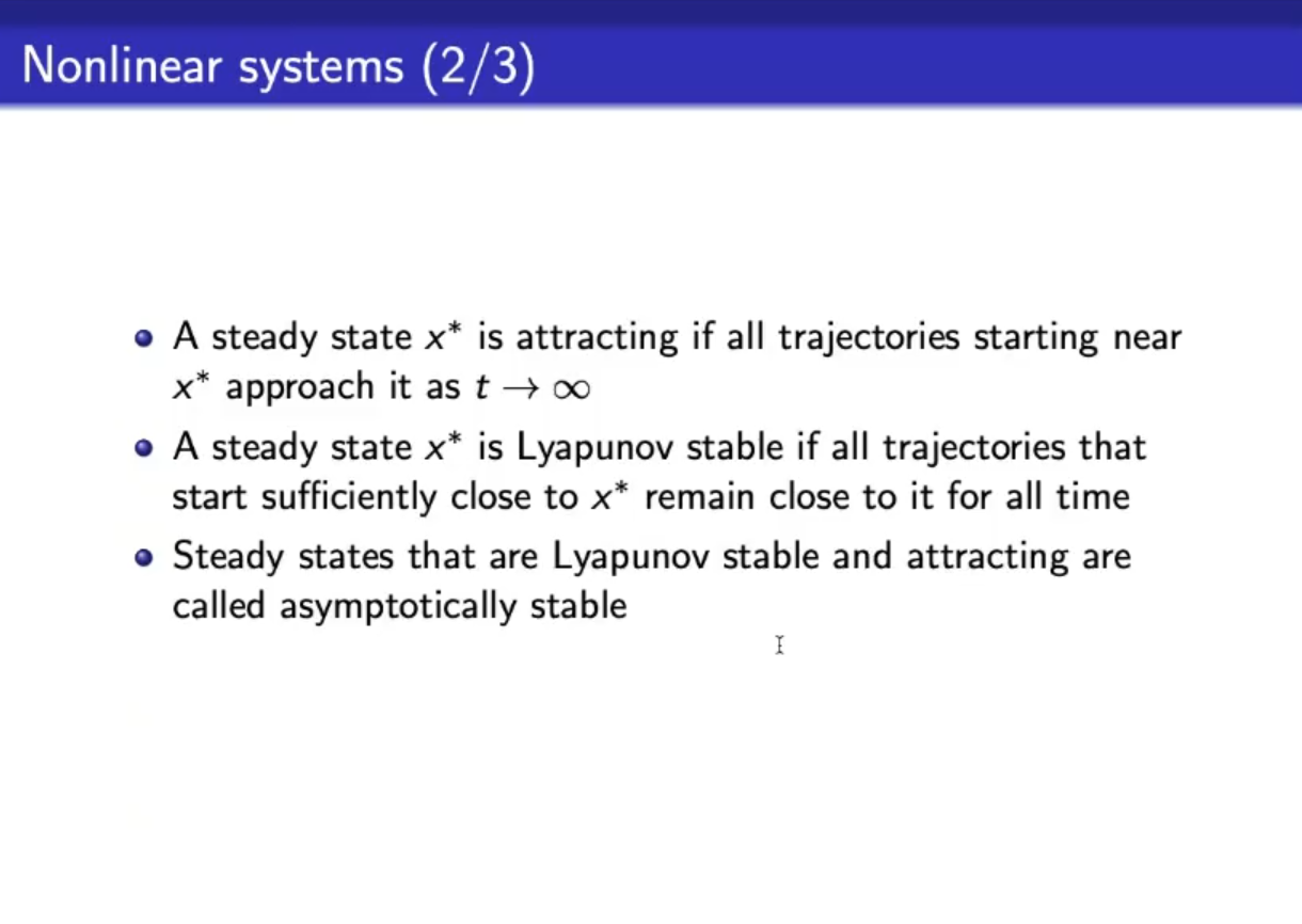
Somenthing i skipped, example of stable and unstable ss: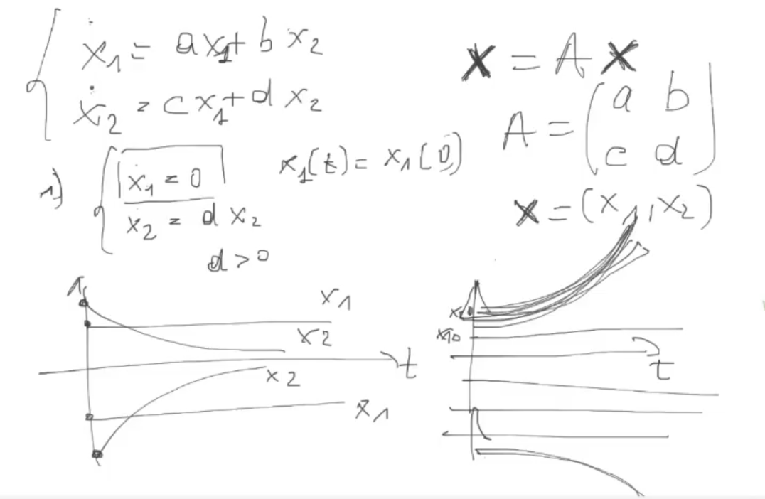

Somenthing i skipped, example of marginally ss: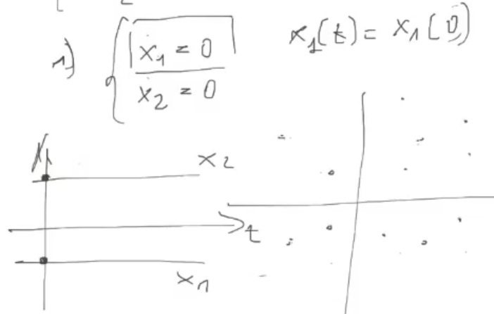

#TODO Repeat the missing part on the lecture

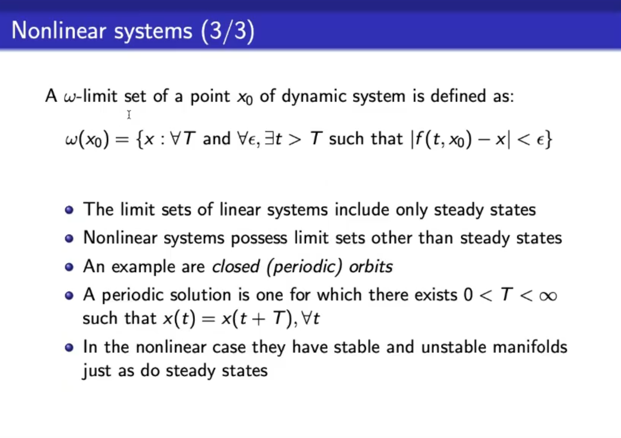
• The “limit cycle” is a robust oscillation, meaning that they are attracting

---

• Recap, basically it exaplains the plot of $\tau$ and $\Delta$, we have seen previously

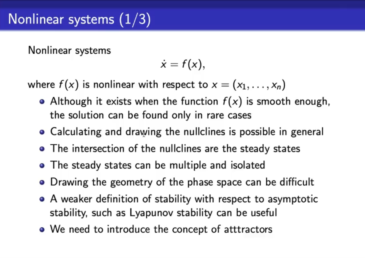
• In non-linear system we will observe that non only points can act as attractors (in linear case the stbale ss act as actractors).
  In non-linear systems there can be closed curves in the phase space that can act as actrators.IMPORTANT
  And there can also be closed curves that do the opposite (like for unstable ss in linear systems)
• You can imagine that in non-linear sytems the steady state can also be closed curves.

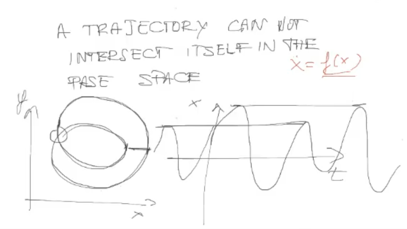
This is a possible phase space of a non-linear system: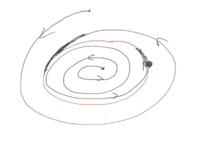

• The red circle acts as an actractor.
• This phase space is impossible to be obtained in a linear system.

And its dynamics: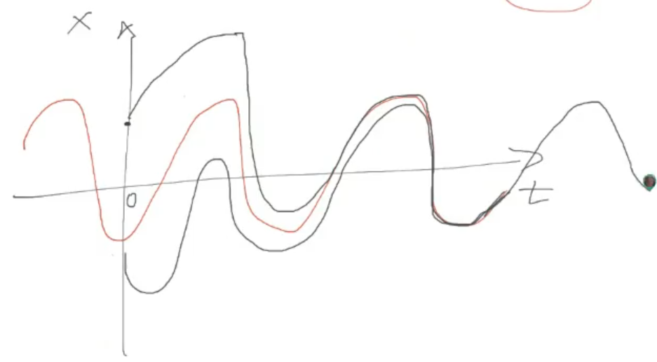

• Actracting curve, robust oscillation.

If we focus on the actractive circle, from an initial condition inside this curve: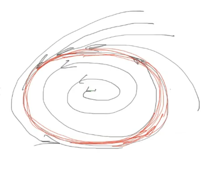

• In red the actractive circle.
• This means that at the center of the circle we need to have a repulsive ss.
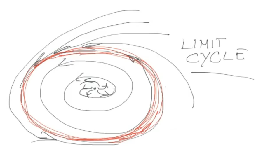
• This actractive curve/circle is called “limit cycle”:
  

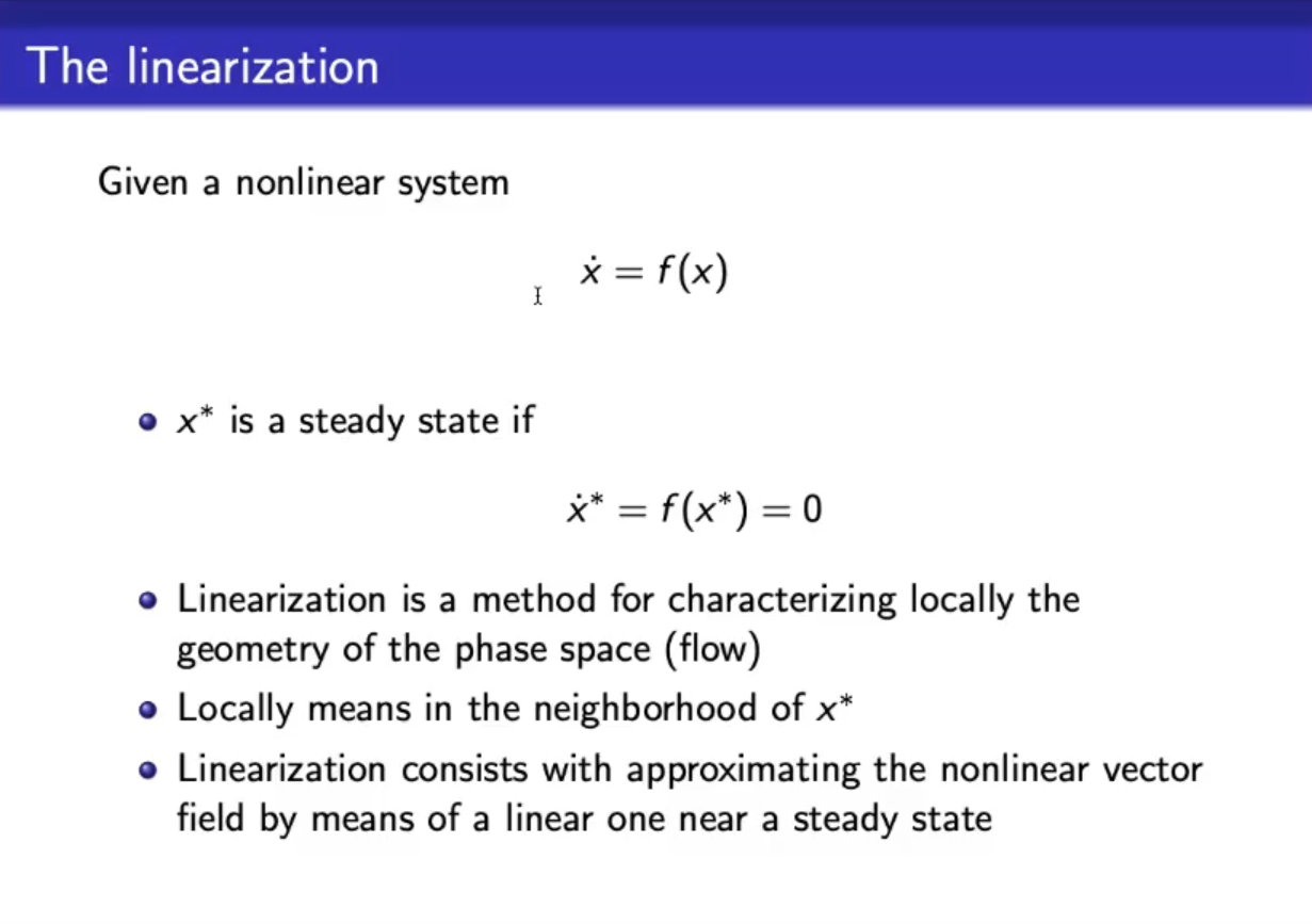
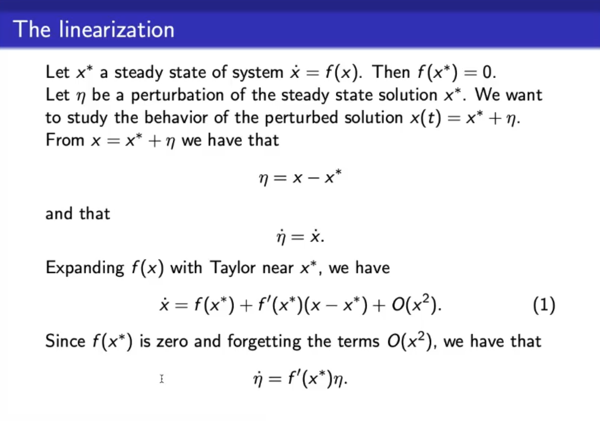
• Mathematical proof and explanation on how we can linarize numerically.

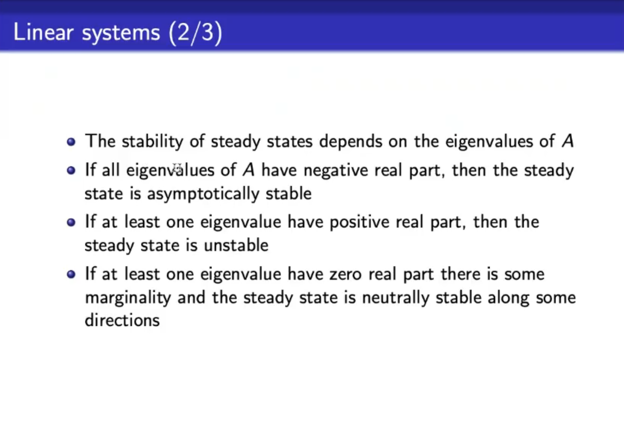
• If the eigenvalues are hyperbolic, then the linearization is “succeful”, mening that both stability and flow are qualitativly the same.
• Non-hyperbolic ss may produce dynamics that are not predicted by the linearized system, so we cannot analyze them via linearization.
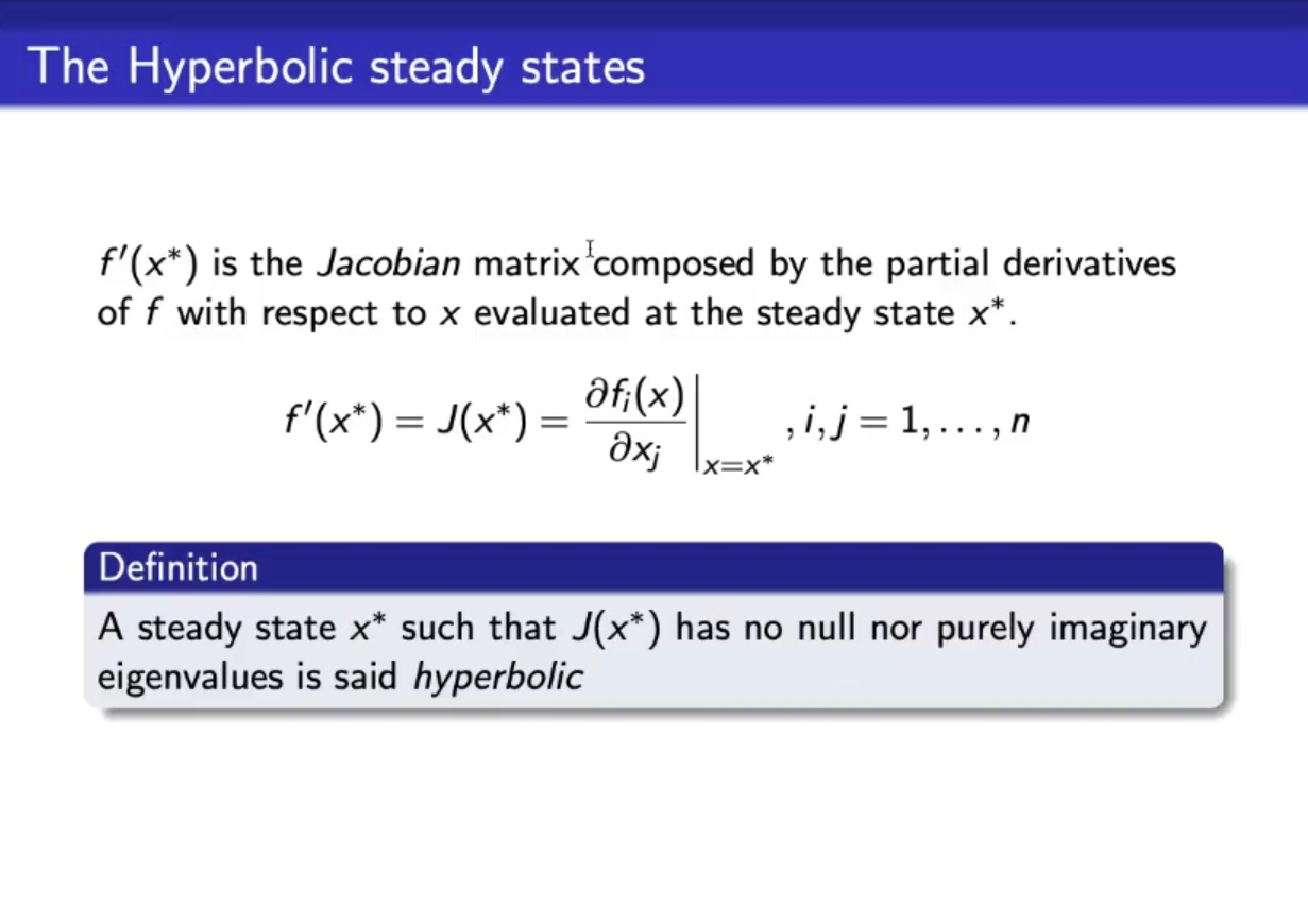
• If all eigenvalues are different from $0$, just looking at the eigenvalues is sufficient to conclude about the stability of the steady states, and also about the geometry of the phase space near the ss
  But if there is at least one $0$-eigenvale, then we cannot predict the geometry of the phase space, near the ss by analyzing the linearized system, we need to use other tools.
• The presence of $0$-eigenvalues may produce a very complicated dynamic, including limit cycles, and also the strange actractors, so we need to study really well the system if this is the case.

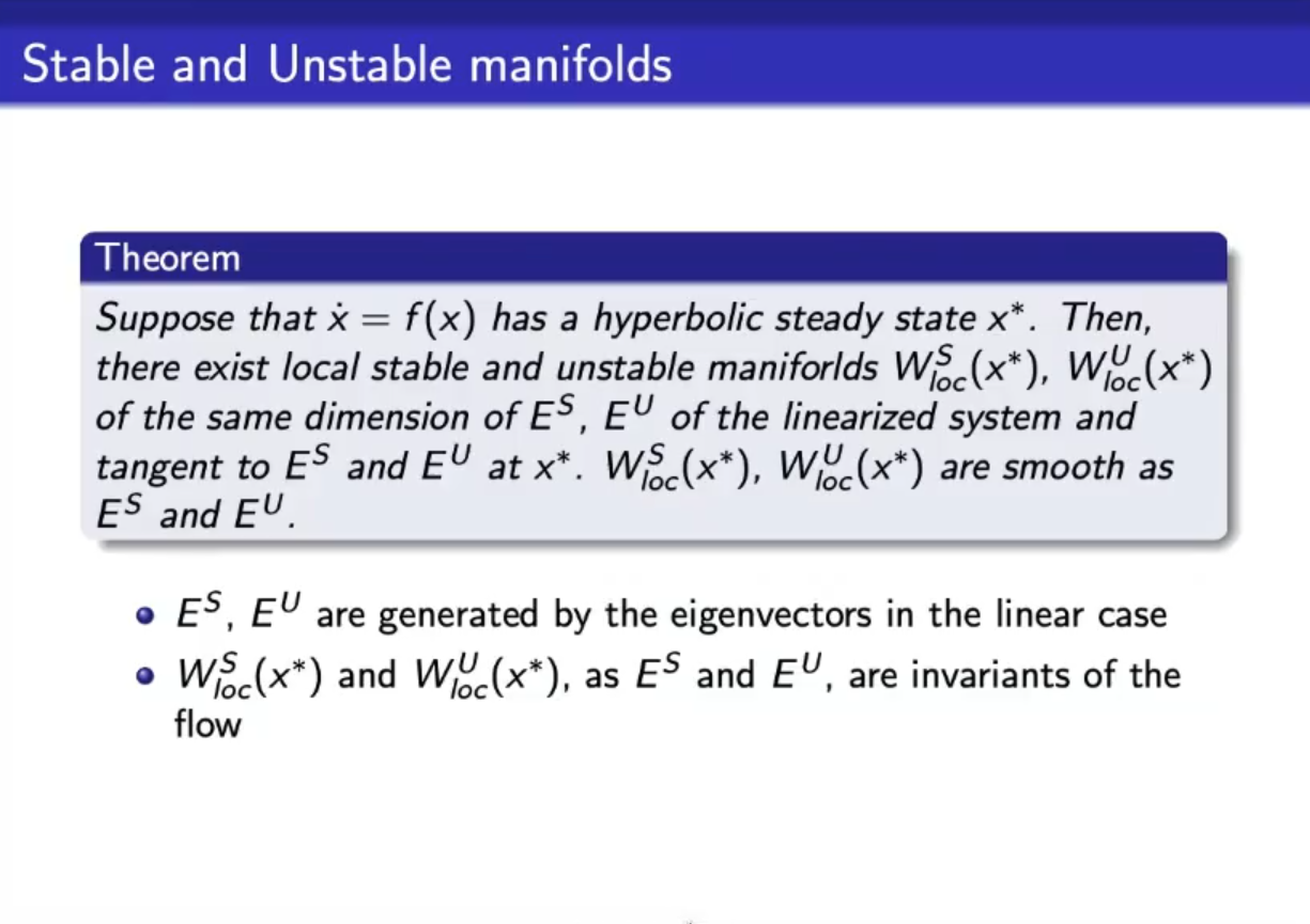
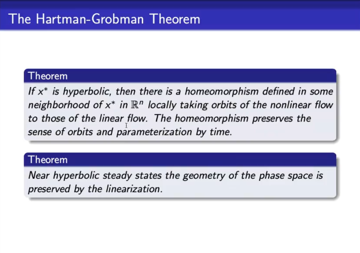
• In case of hyperbolic steady states, not only the property of stability of the ss are similar in the non-linear and linearized system, but also the geometry nearby.
• Also in the non-linear case we can distinguish between stable and unstable manyfolds (or subspaces).

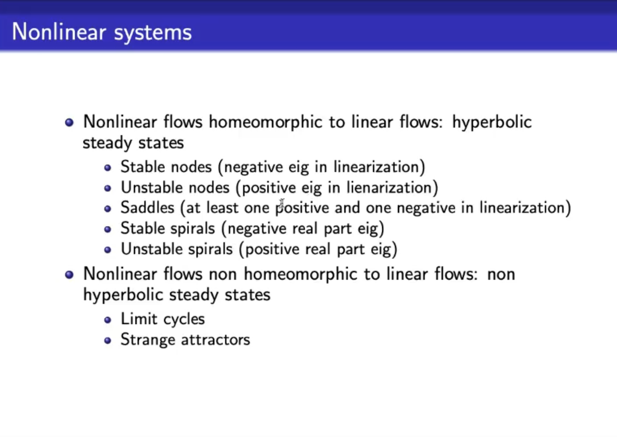
• stable/unstable nodes, saddles, and stable/unstable spirals can be succefully analyzed via linearization.
• limit cycles and strange actractors cannot.