CDS - Lecture 12

• $T_1>T_2$
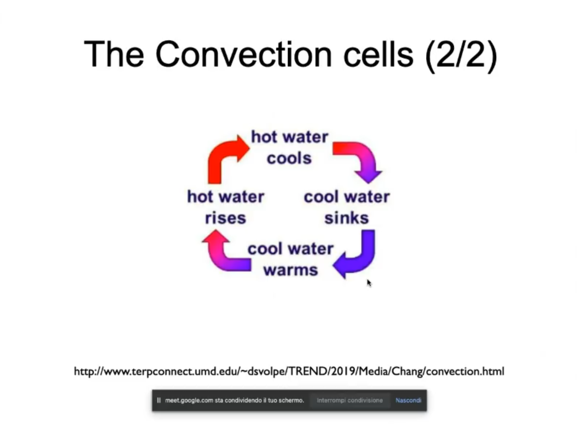
• This is a somewhat of an “organization” (not compleately chaotic).

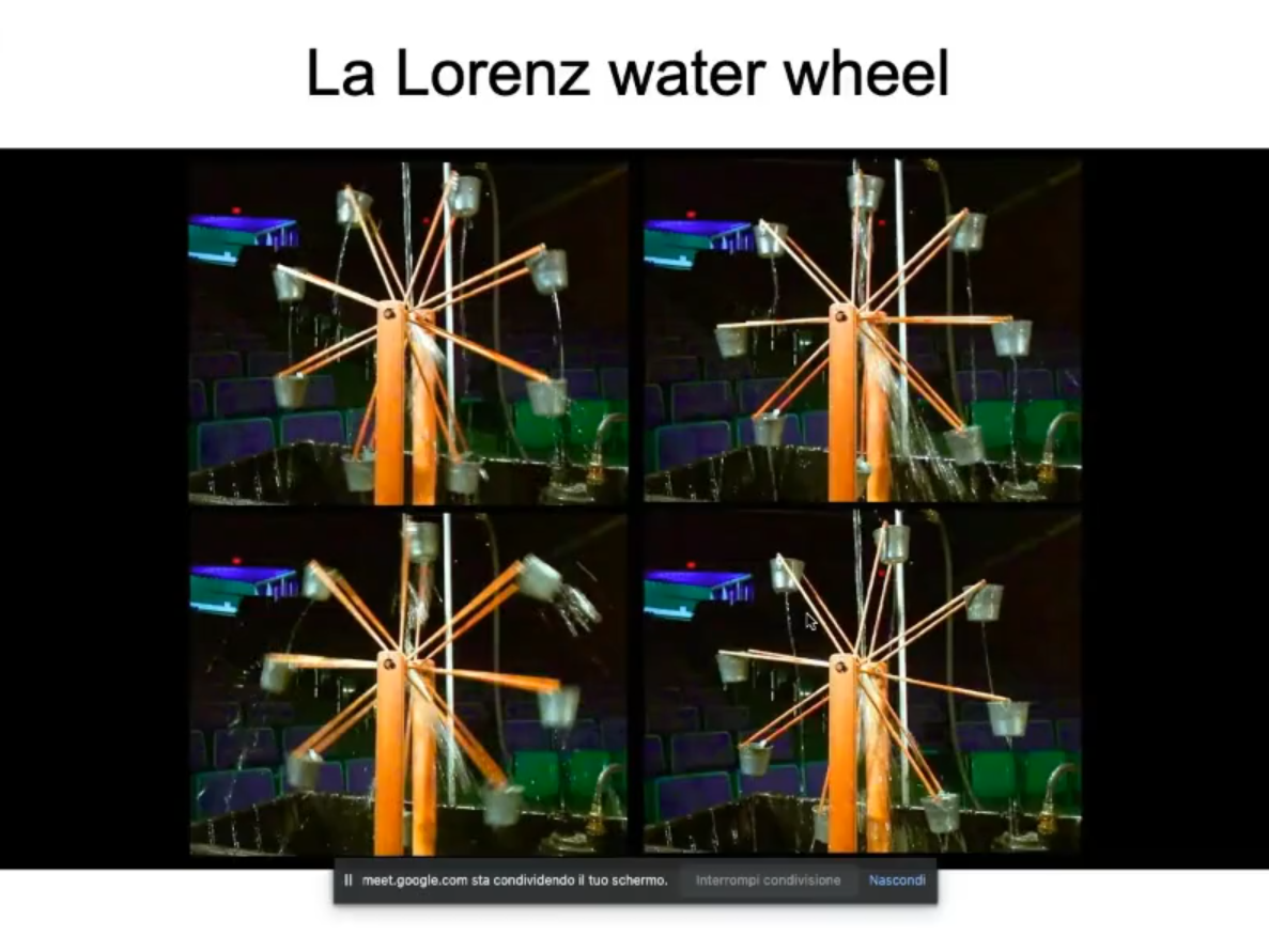
• The four weels will evolve differenty (sensitivy to inital conditions)

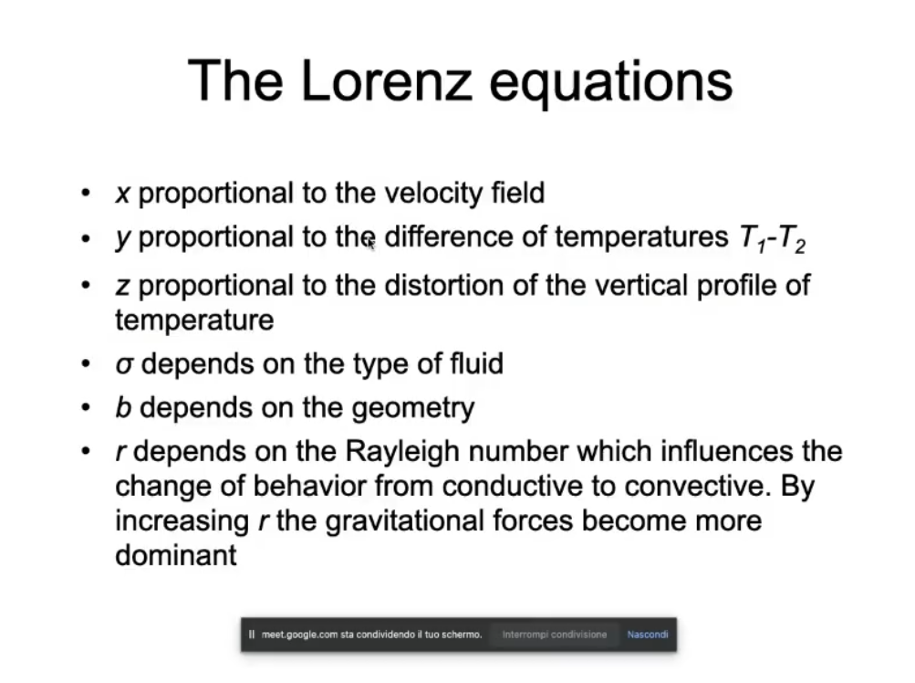
• Autonomous (no external forces influence the system)
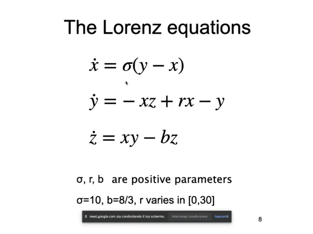
• Almost linear (we only have $xz$, and $xy$ as non-linear terms)
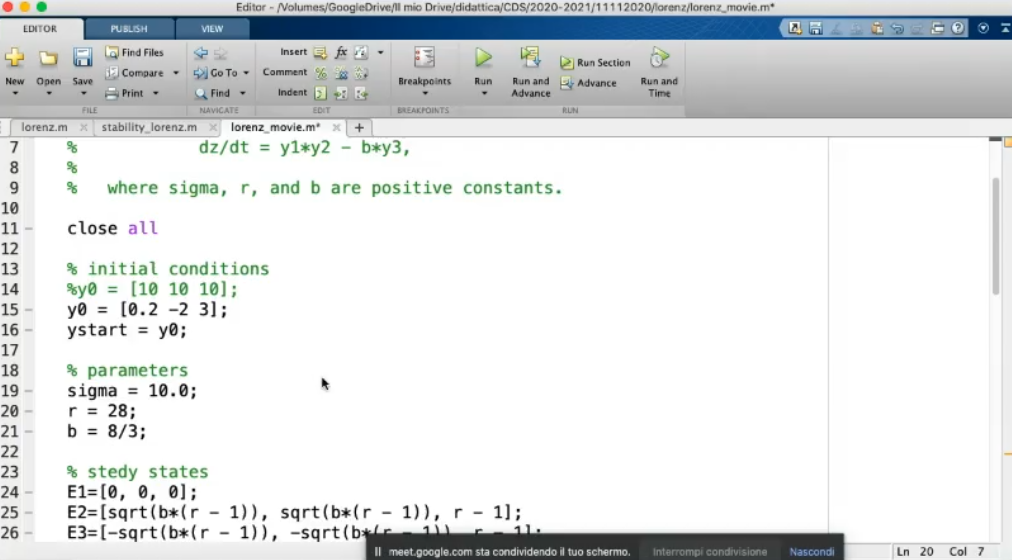
• We fix $\sigma$ and $b$ and study the system for $r\in \left[0,30\right]$.

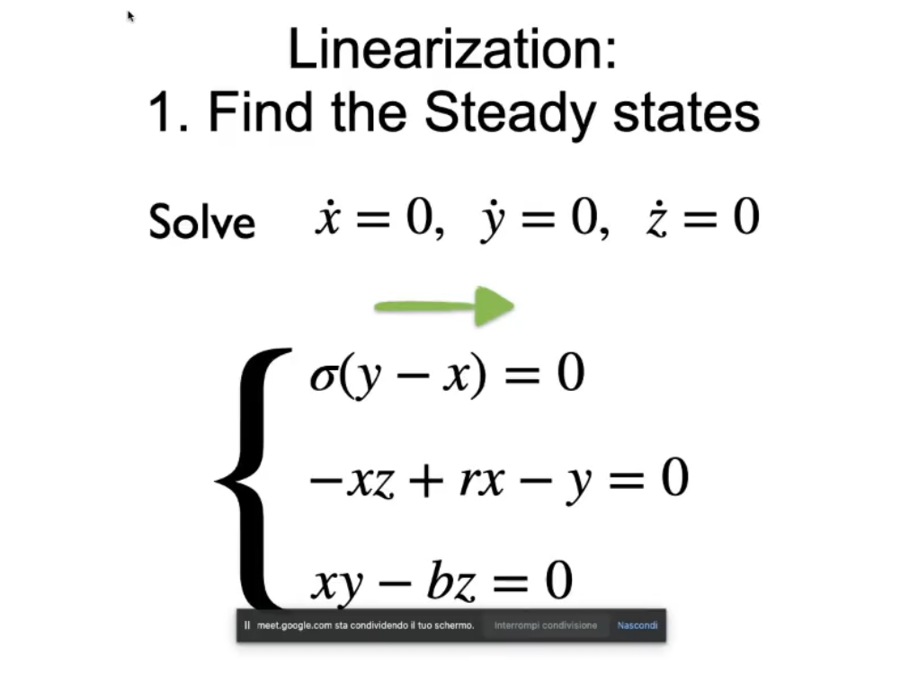
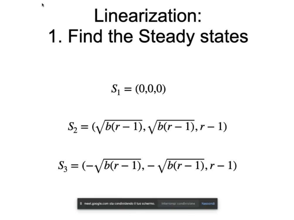
• We find $3$ steady states.

• Remeber that “linearization is a local process”, so we’ll need to repeat the following process for each steady state.

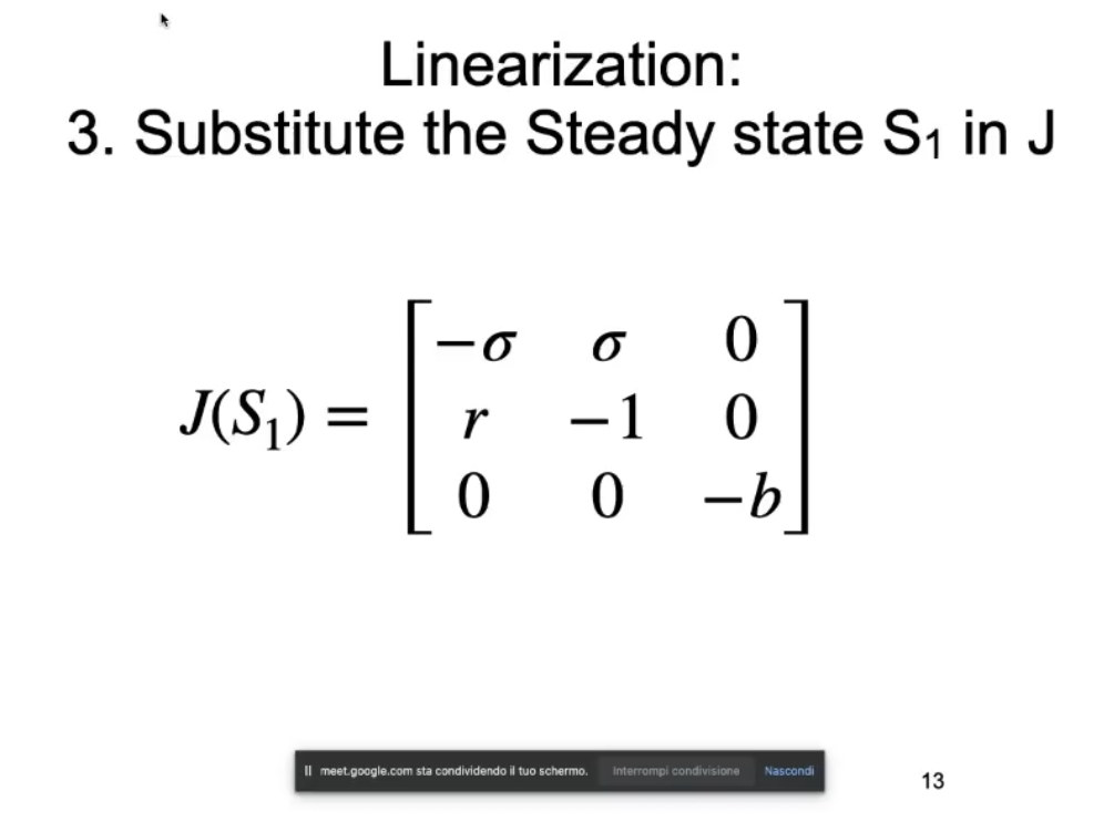
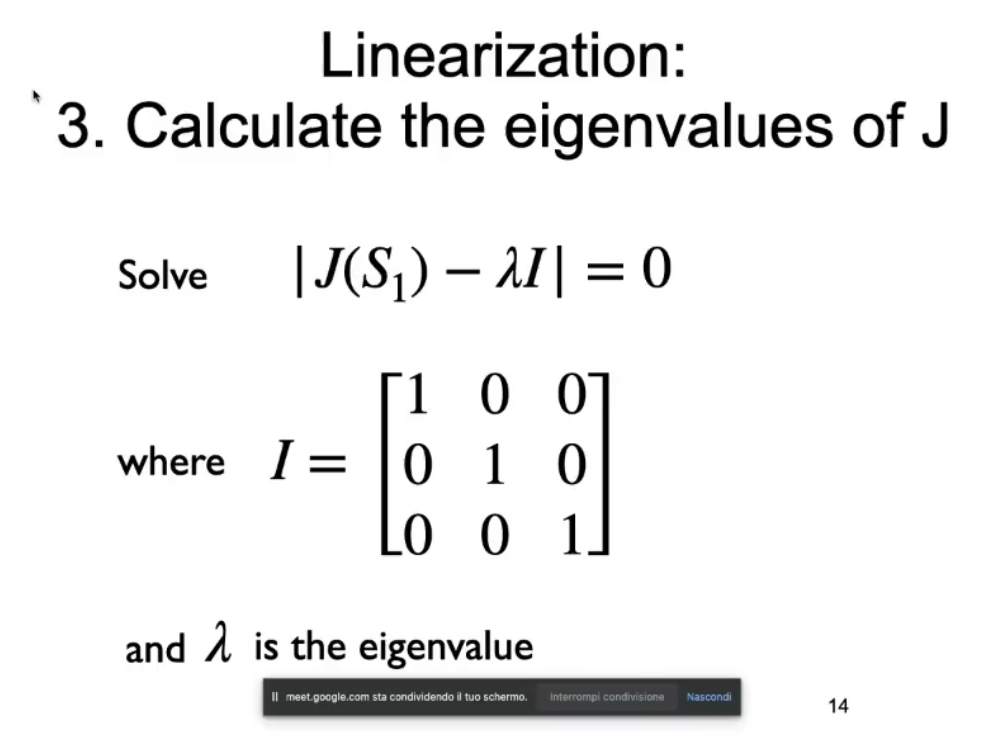
• Remeber that: $S_1=\left(0,0,0\right)$

• bifurcation diagram.not-sure-about-this

• Remeber that: $S_2=\left(\sqrt{b(r-1)},\sqrt{b(r-1)},r-1\right)$
• Remeber that: $S_3=\left(-\sqrt{b(r-1)},-\sqrt{b(r-1)},r-1\right)$

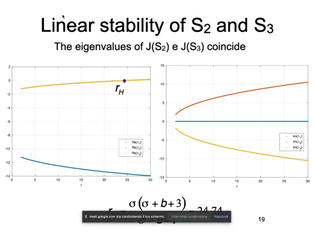
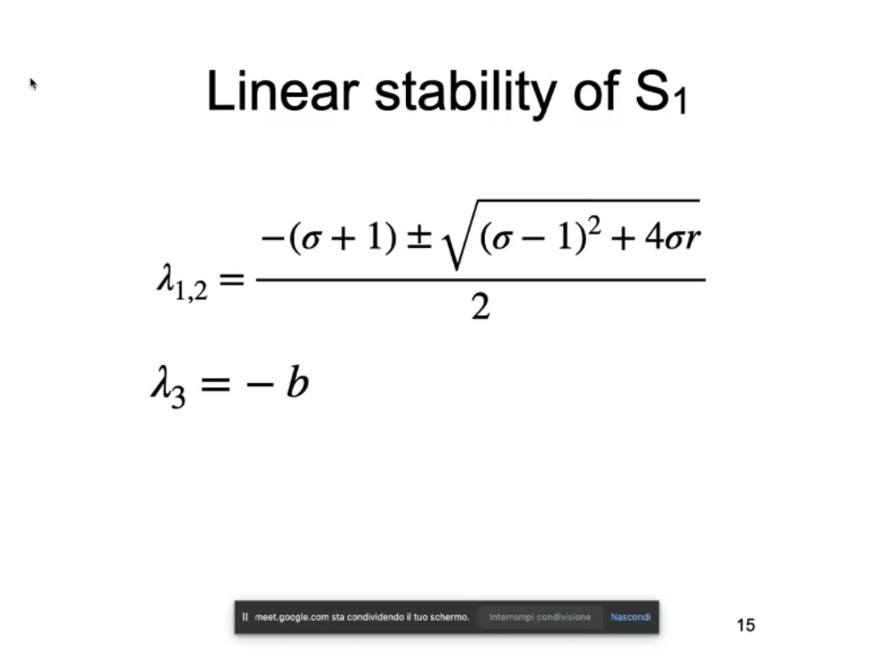
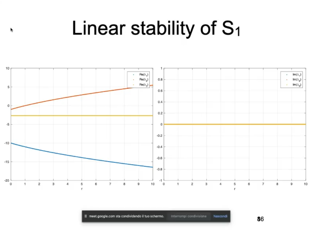
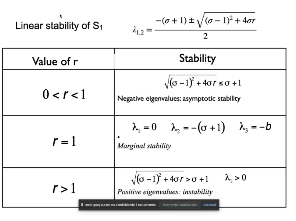
• The have non-zero imaginary part.
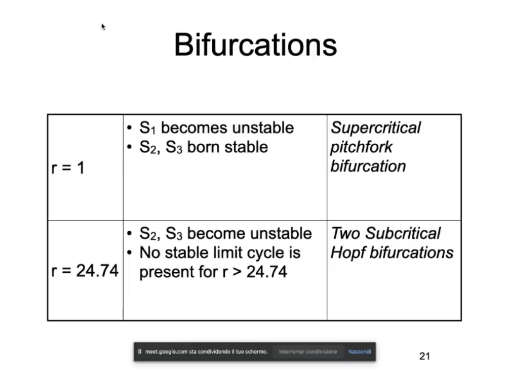
• For $r\in \left[1,\sim 24.74\right]$ the real parts of the eigenvalues are negative.
• $\mathrm{Re}({\lambda }_1)=\mathrm{Re}({\lambda }_2)$.
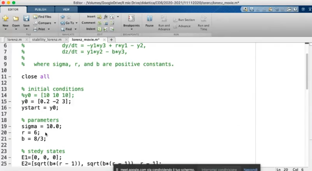
• For $r<r_H$ (called “critical value”) then the system is stable.
• For $r>r_H$ the system is unstable.
• For $r=r_H$ the real part of the 3rd eigenvalue $\mathrm{Re}({\lambda }_3)=0$.
• $r_H\simeq 24.74$ found using MATLAB

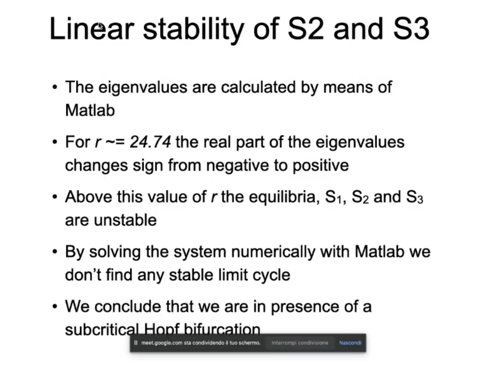
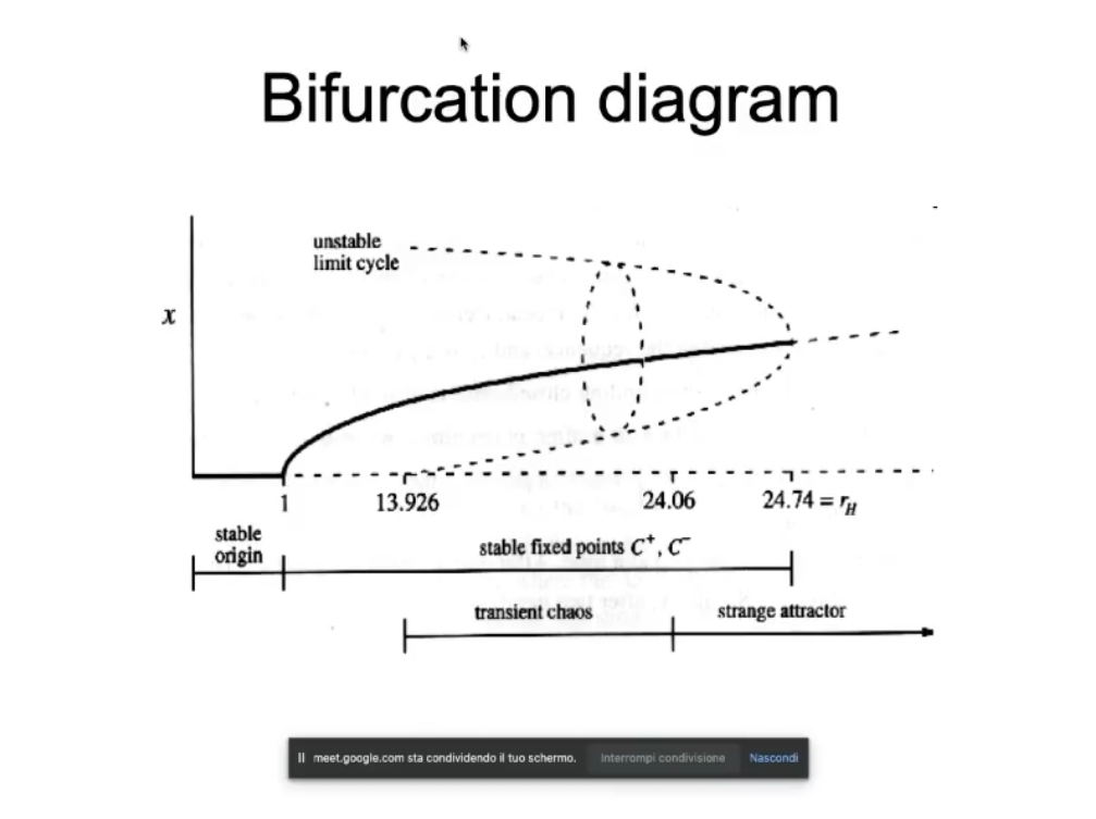
• We don’t see in this picture but there is another unstable limit cycle mirrored with respect to the abscissa.
• NOTE: above $r_H$ we have no stability exist/no attractors.
  Unstable for the linearization ⇒ unstable for the real system.

• $r=0.4$.

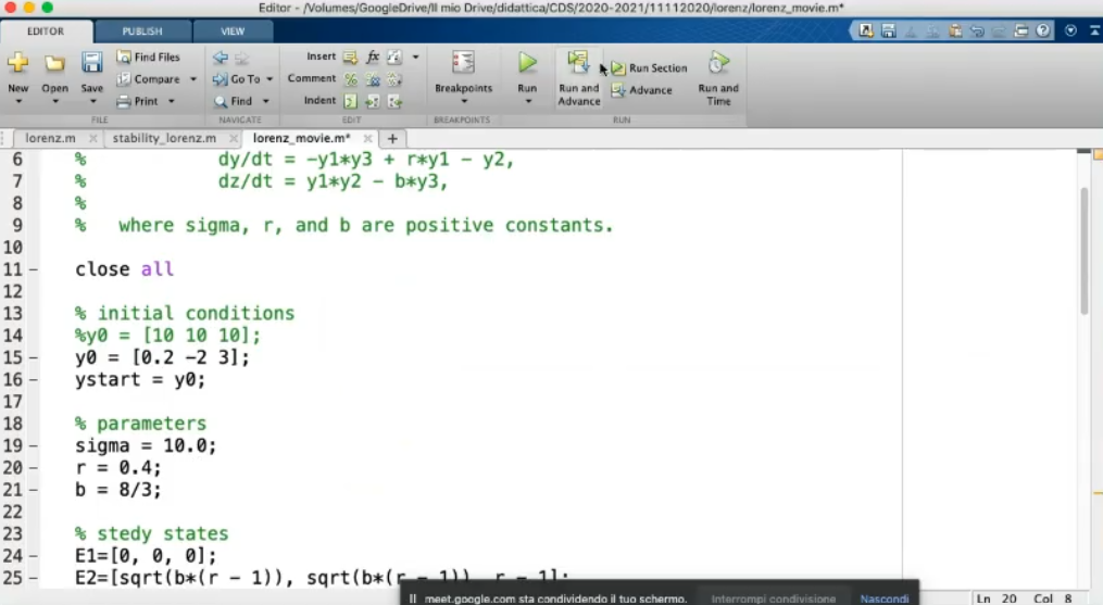
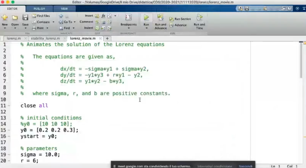
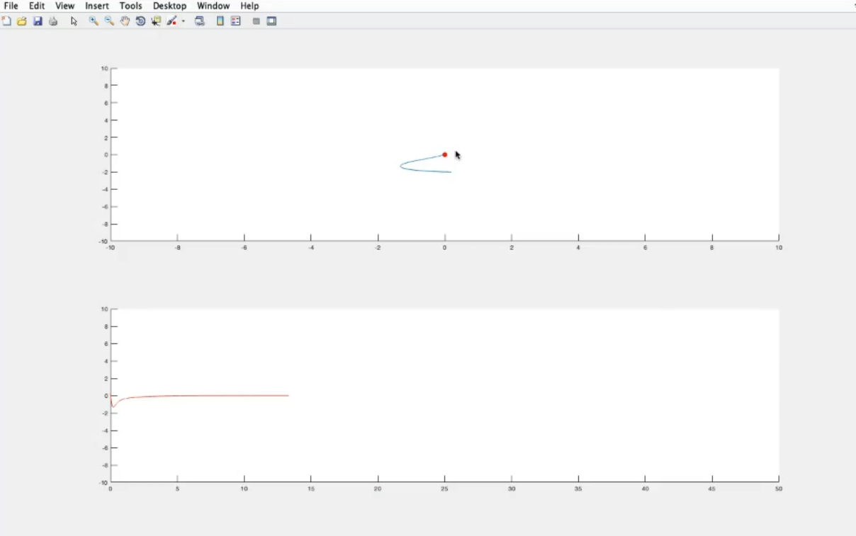
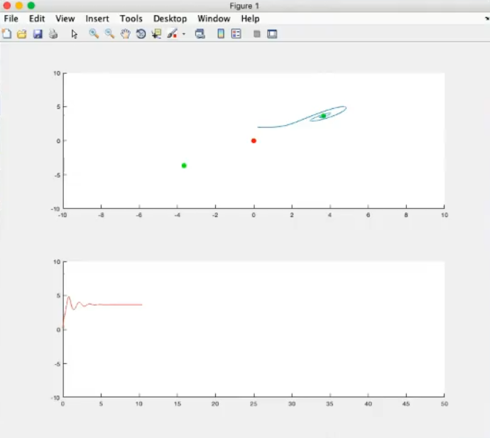
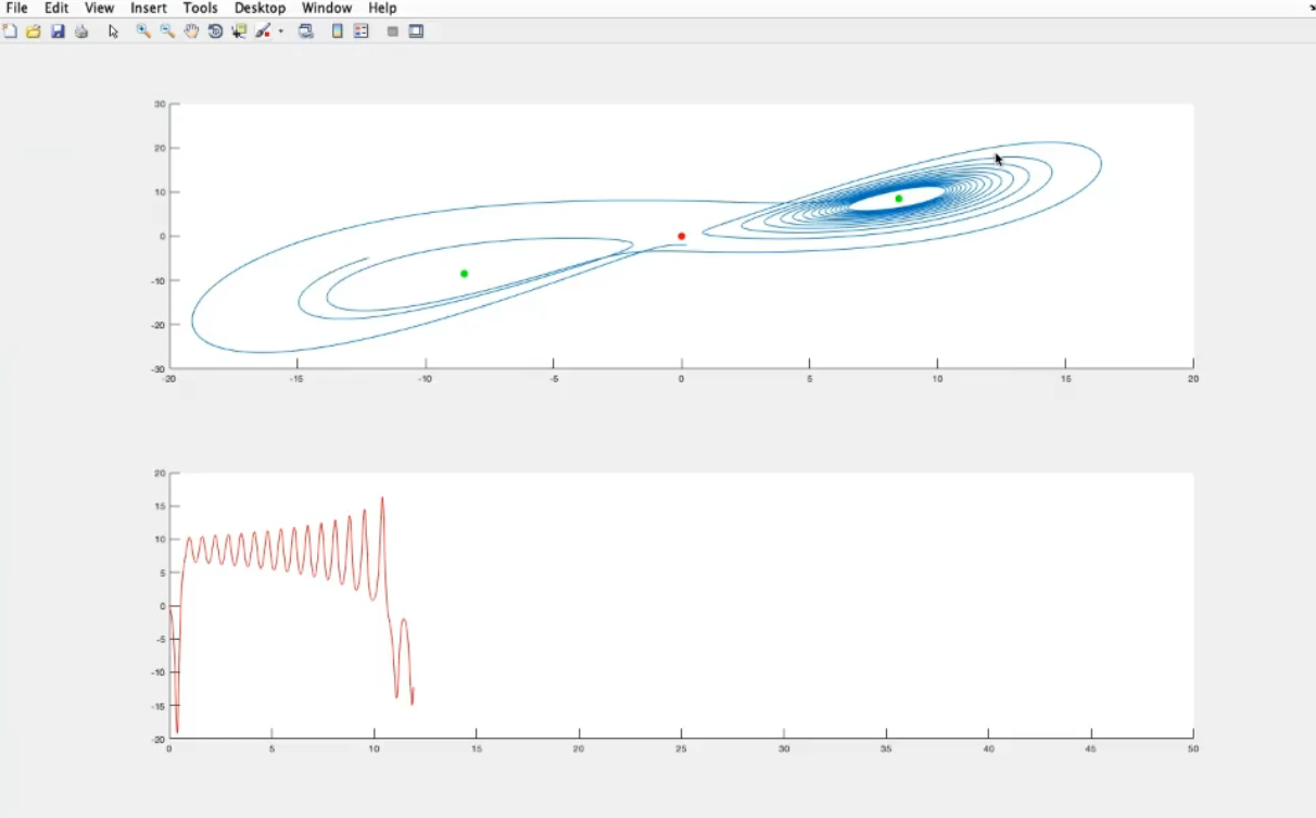
• Output of the previous, code:
  • In the first subplot we represent the phase space.
  • In the second subplote we represent the dynamics.

• $r>1$ (specifically $r=6$)

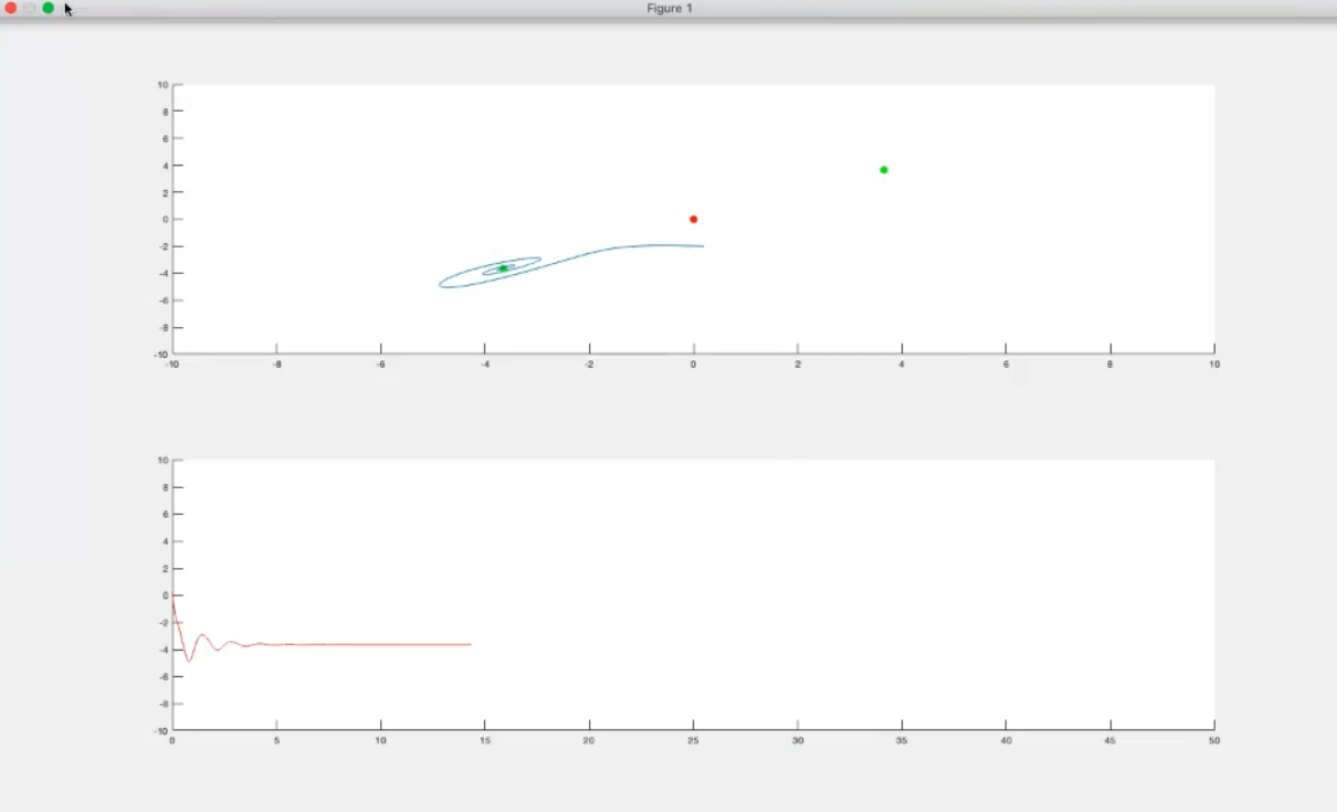
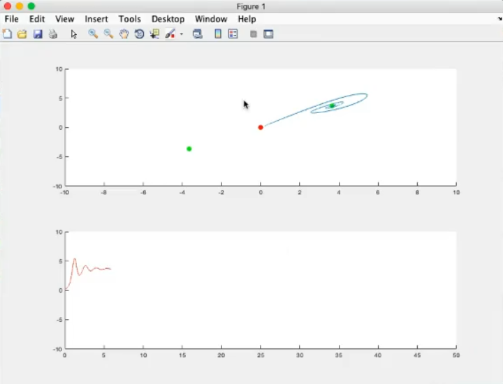
• Output of the previous, code.
• The origin is now an unstable steady state

• We change the initial conditions, $y_0=\left[0.2,2,3\right]$

• We now converge to the second stable steady state.

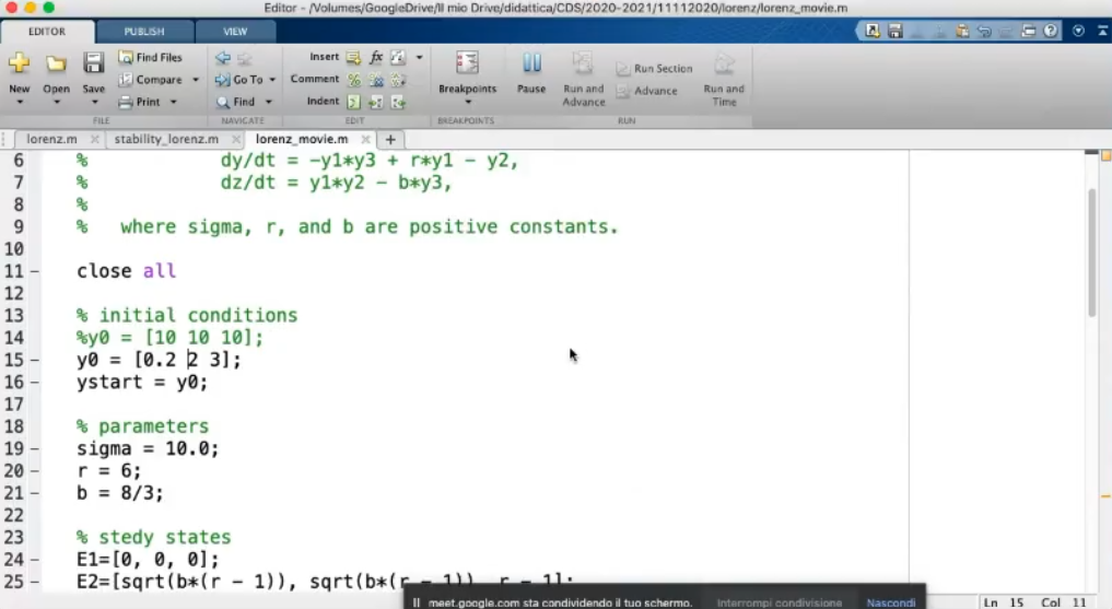
• We change the initial conditions, $y_0=\left[0.2,0.2,0.3\right]$ (closer to the origin)

• $r=10$.

• $r>r_H$ ($r=28$)

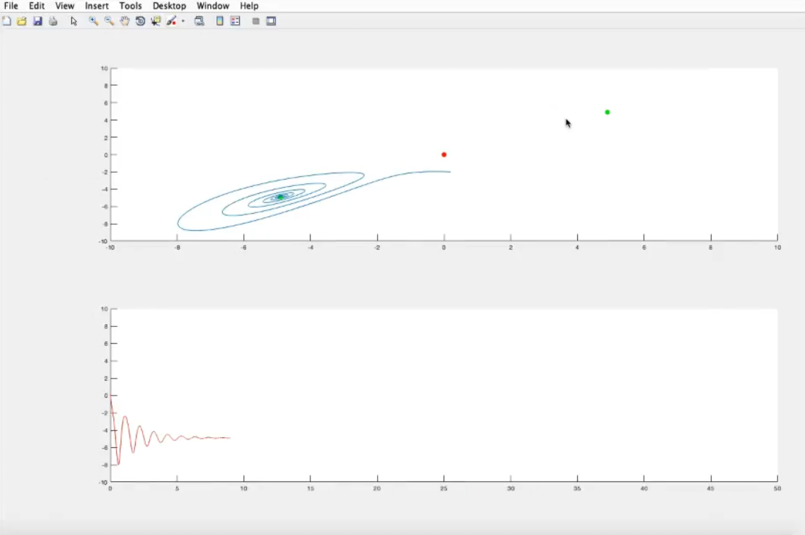
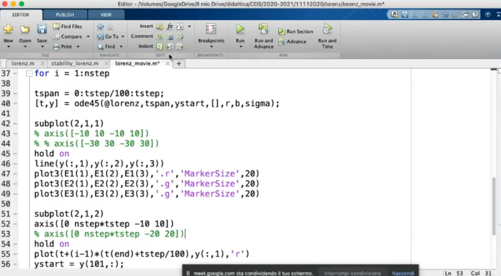
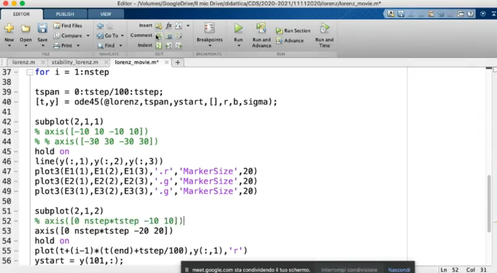
• Also we change the scale of to the abscissa and ordinate.
• (comment axis([0 nstep*tstep -10 10]))
• (uncomment axis([0 nstep*tstep -20 20]))
• (comment axis([-10 10 -10 10]))

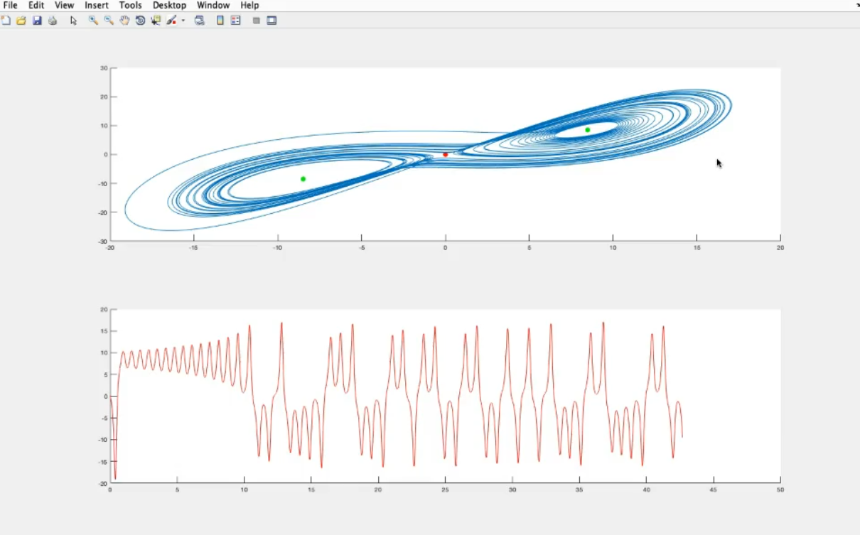
This is the evolution of the chaotic system: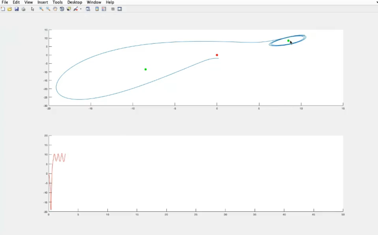

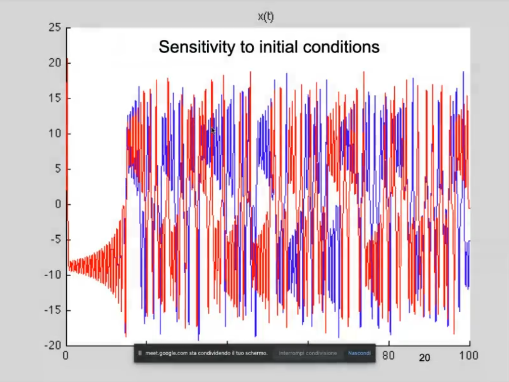
• Sensitivity to inital conditions, we report only one varible ($x(t)$), and 2 sliglty different initial conditions, as you can see thy become compleately different after some time, even if they started really close to one onother.

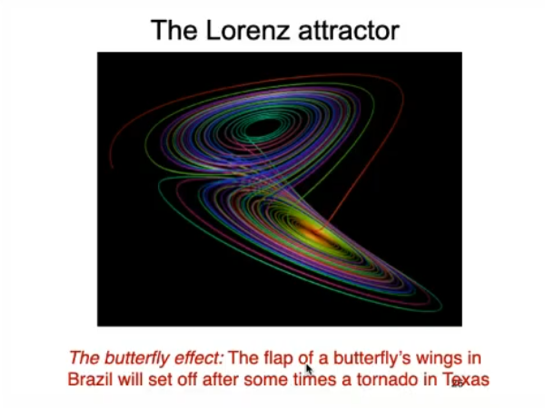
• A very very tiny change of the inital conditions, will produce an enormous change in the system after some time.
• It is called an attractor, since the system will not diverge, it will remain confined in a closed region.
• It is also called “strange attractor”, because ins not a typical one, the typical one are:
  • stable steady states (atttractors)
  • limit cycles (and multiple-period limit cycles)

Rememebr that this is a 3D object: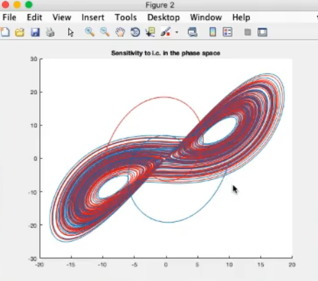

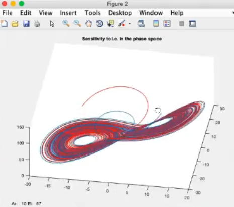
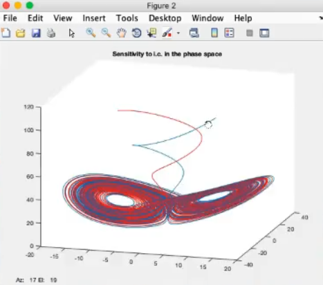
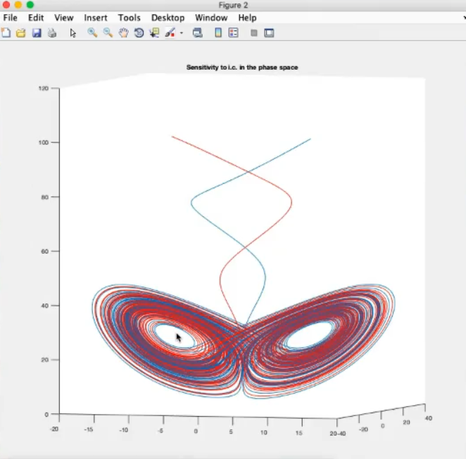
• The two circles are unstable steady states.
• In the middle of the two unstable steady states we have the origin $\left(0,0,0\right)$.