CDS - Lecture 8

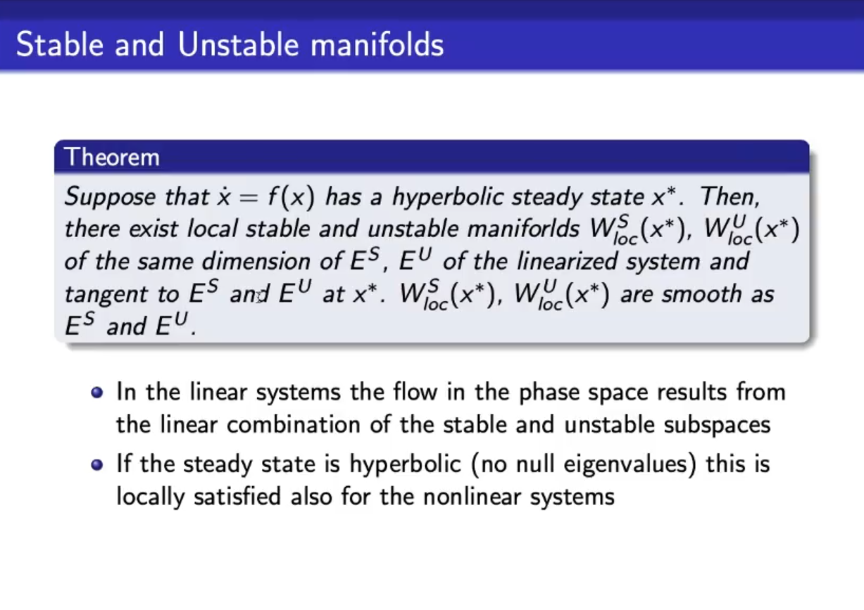
• hyperbolic ss: the associated linearization does not have any $0$-eigenvalues, meaning the all eigenvalues are $\ne 0$, or in case that they are imaginary, their real part is $\ne 0$.IMPORTANT
• A manyfold is a generalization of a subspace in a nonlinear space.IMPORTANT
• ${}^U$ : unstable
• ${}^S$ : stable
• The manyfolds $W$ are tangent to $E$ specifically at the stady state $x^{\ast }$, this means:
  1. We can approximate a non-linear system into a linear system, and we get similar information regarding the stability of the stady states (if the ss is hyperbolic).
  2. In linear systems, the subspaces $E^S$ and $E^U$ generate/span the whole phase space, meaning that any vector is a linear combination of the vector spanning $E^S$ and $E^U$.
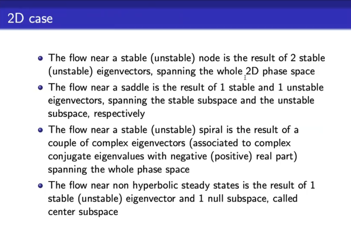
     For example, if you have only stable subspaces ⇒ then you will have only stable steady states.
     ==$E^S$ and $E^U$ are generated respectivly by negative and positive eigenvalues/eigenvectors==.

This is the space generated by eigenvector with both positive eigevalues: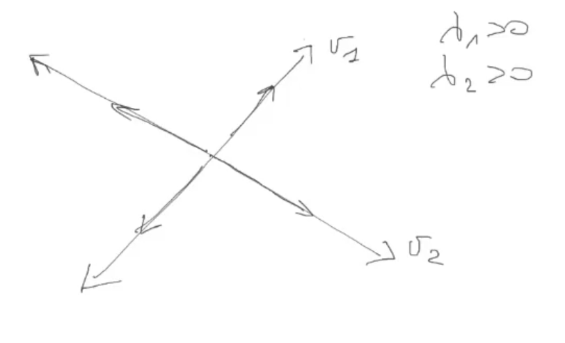
And the flow associated is:

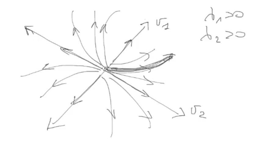
Example of a saddle (linear):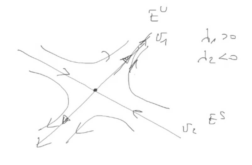

• $v_1$ spans the unstable subspace $(E^U)$
• $v_2$ spans the stable subspace $(E^S)$

Example of a non-linear saddle: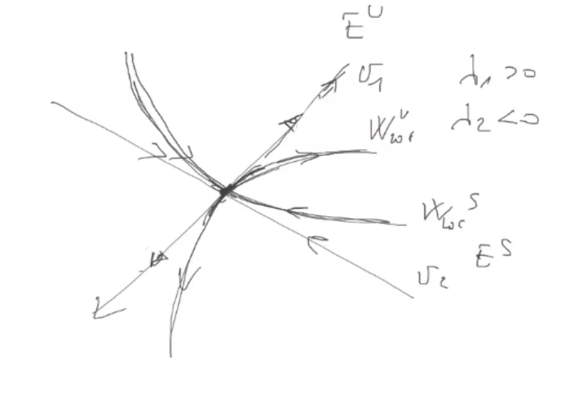

• near to the ss, the linar approximation is tangent to the manyfold
• As you can see the stable manyfold $(W_{\text{LOC}}^S)$ has the flow that points toward the ss, while for the unstable manyfold $(W_{\text{LOC}}^U)$ the flow points to infinty.
• The linar approximation is valid only near the ss.

If we draw the flow of the non-linar system: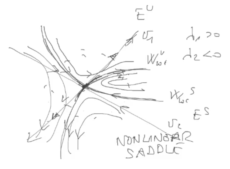

• Notice the similiraties with the linear system.
• In this case is like the linear system, but it is distorted.

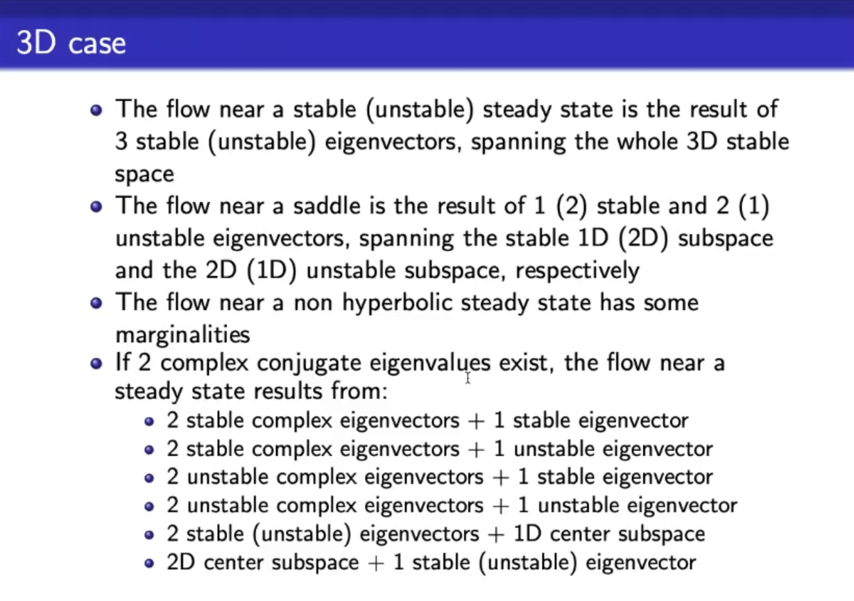
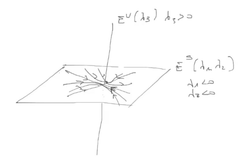
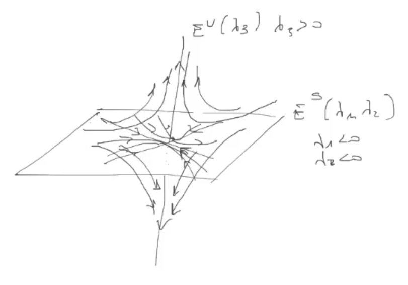
Example of a “3D saddle”, however this is not the “official name”, in 3D we don’t distinguish between “nodes”, “spirals”, “saddles”, …:
In general this is referenced as: “2 stable, 1 unstable eigenvectors/eigenvalues”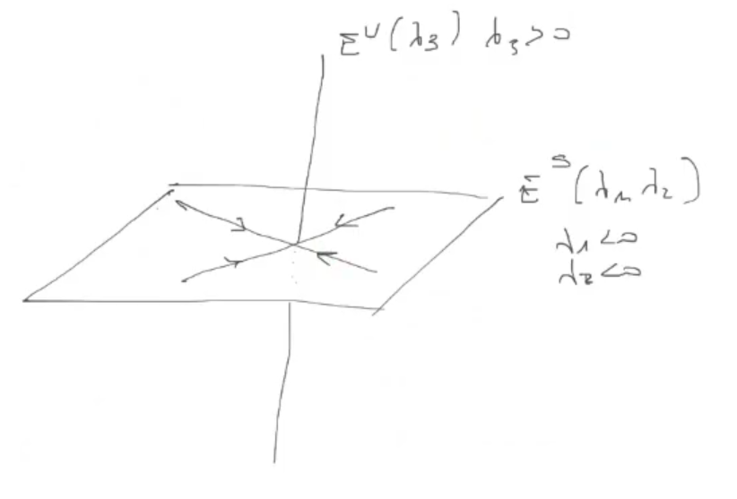

Example of 2 stable imaginary conjugate, 1 stable eigenvectors: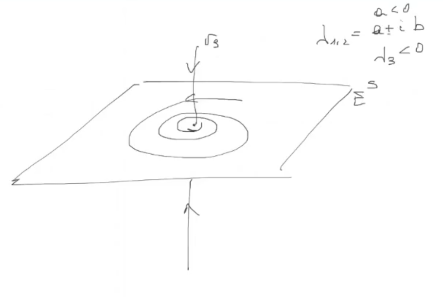

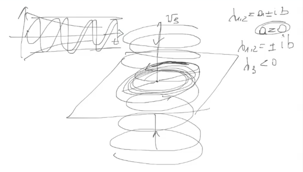
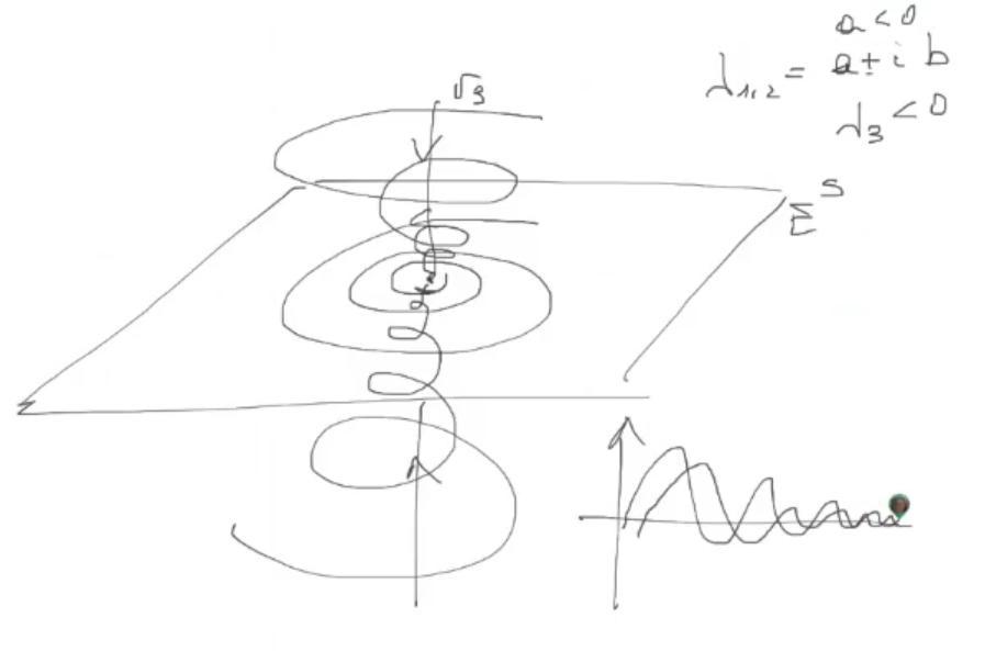If instead we have 2 stable imaginary conjugate, 1 unstable eigenvectors:

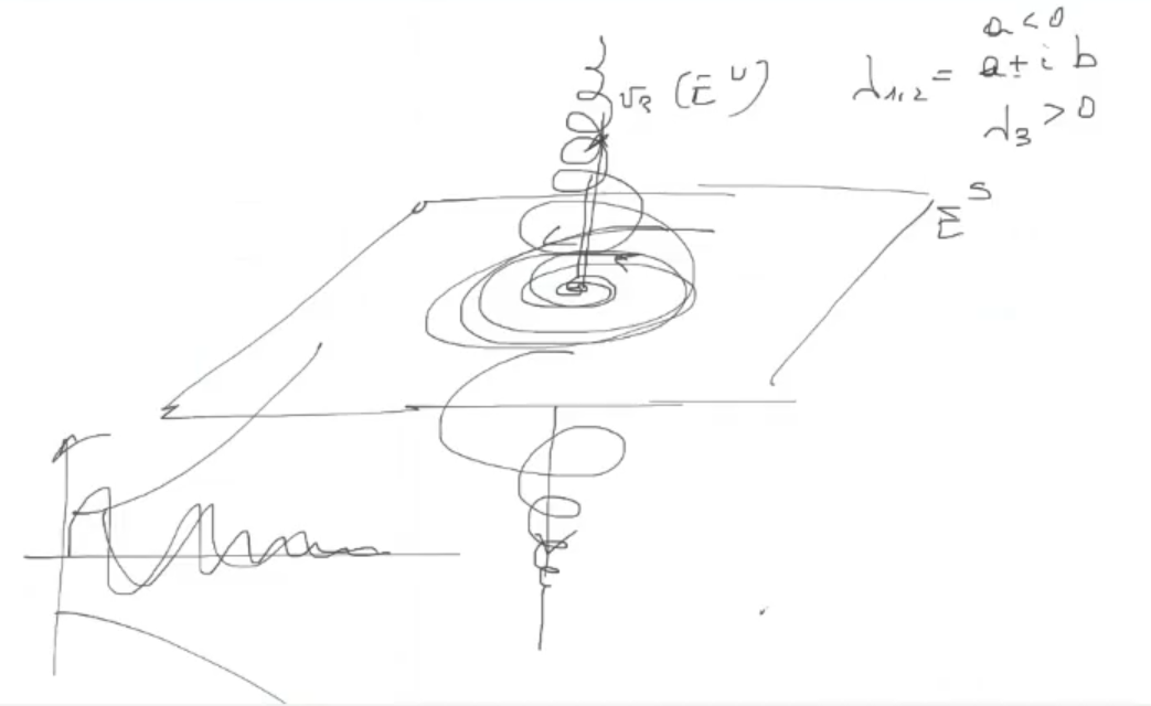
• Notice how in the phase plane the two conjugate eigenvalues converge to $0$, but the third one diverges.

2 marginally-stable imaginary conjugate, 1 unstable eigenvectors: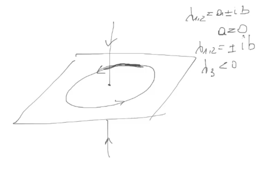

• In the phase plane we have 2 sinusodial “constant” function (their amplitdue reamains constant) and 1 exponentially decreasing function.

If instead we have 2 marginally-stable imaginary conjugate, 1 marginally-stable eigenvectors: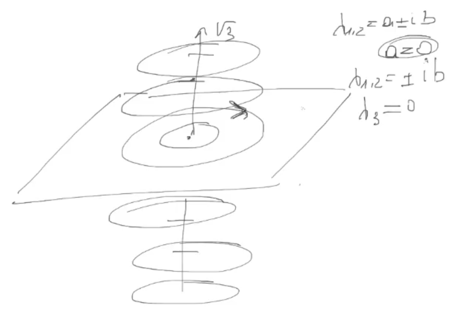

• This is an infinite series of separated circles.

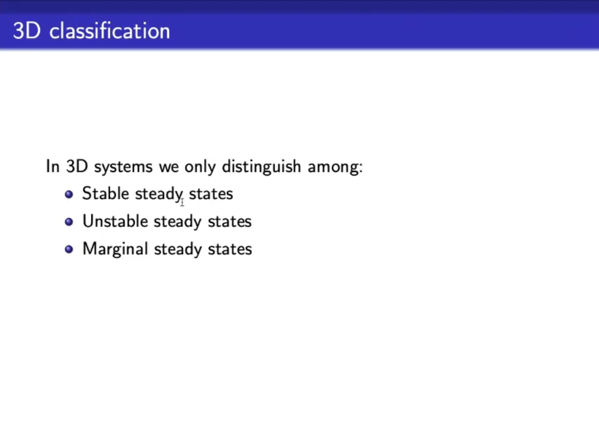
• In 3D we don’t distinguish between “stars”, “nodes”, …

---

• ~Ex.: steady states that disappear when changing the parameters.
• If in a system all ss are hyperbolic ⇒ the system is structurally stable.
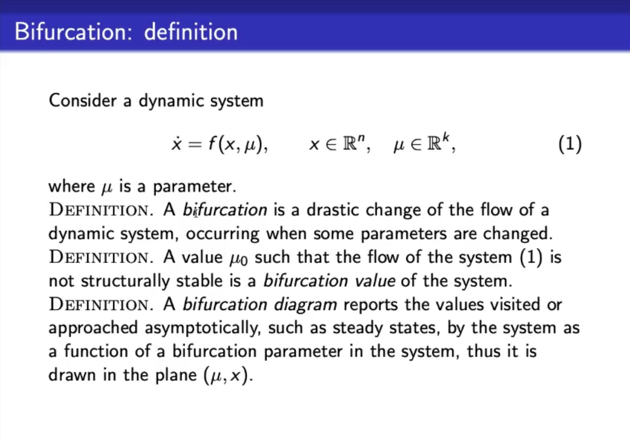
• To have structural instability we need that chagning the parameter we change the sing of the eigenvalues, at the value of the parameter, for which we have the change of sing, so for ${\mu }^{\ast }:{\lambda }_1\text{ or }{\lambda }_2=0$, we have a “bifurcation” ($\mu$ is the parameter)

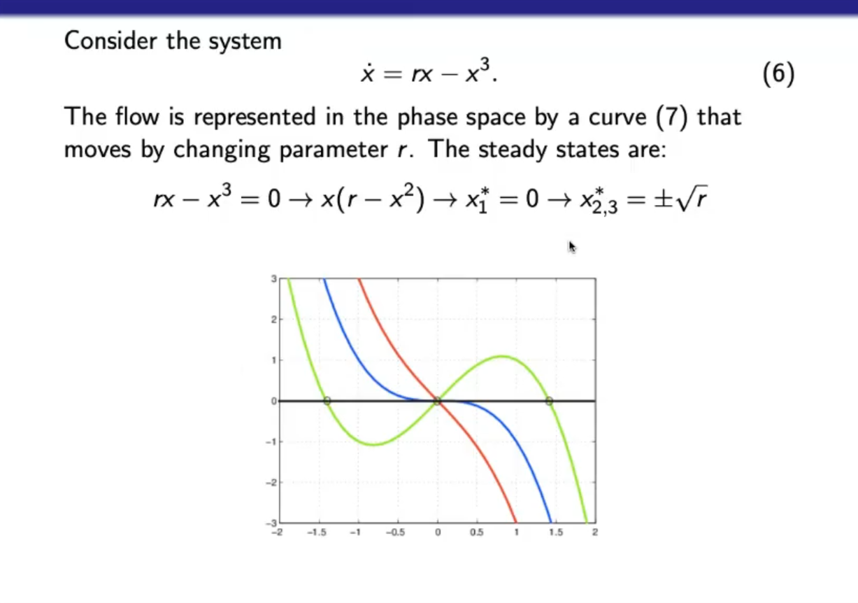
• $f$ is a non-linear function.

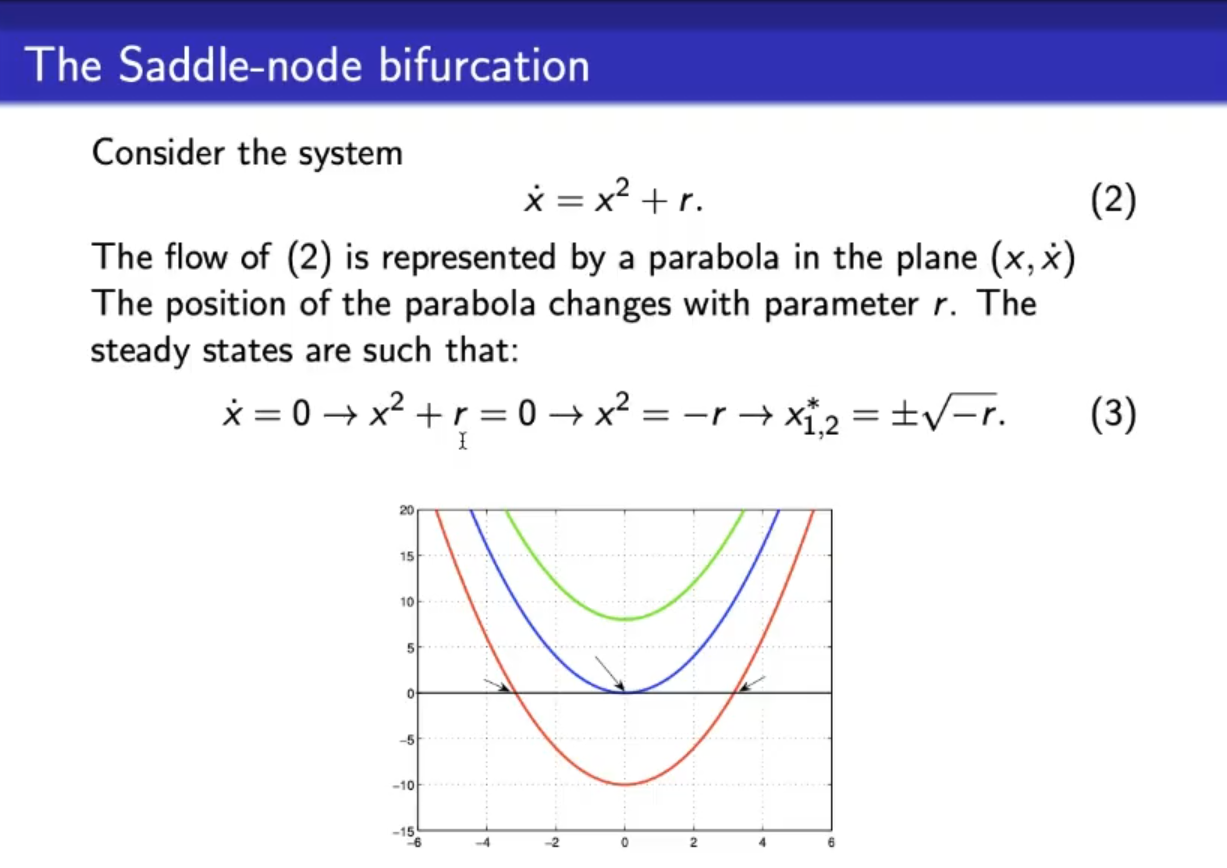
• This graph is NOT the “bifurcation diagram”, we will see it later.
• The arrows in the diagram represnt the steady states, depending or $r$ we may have $2$, $1$ (actually $2$ “coinciding” steady states) or $0$ steady states.
• If we analyze this steady states, like we have seen in the previous lectures, we can see that (looking at the red curve), we have 1 stable ss and 1 unstable ss.

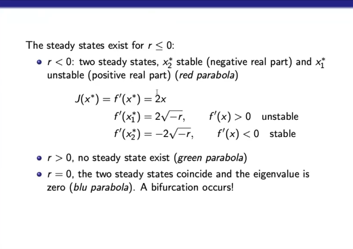
• So for $r=0$ we have a bifurcation.
• Also not that for $r=0$ we have a marginal system/we are in a marginal systuation.
  You can imagine the two steady states (for the red curve, that are 1 stable and 1 unstable) uniting giving un a mix between a stable and unstable ss, however this does not mean that it’s a marginal ss, more on that later.

Let’s see how we analyzed the steady states on the red parabola: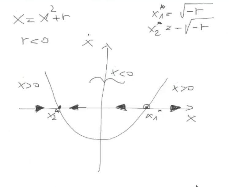
If we perform the linearization:

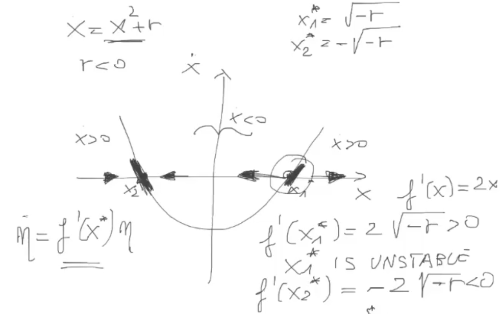
REMEMBER: in a non-linar system you may have no steady state, while in a linear system you have at least 1 ss.

For $r>0$:
We have no steady states.

For $r=0$, the approximation is marginally stable: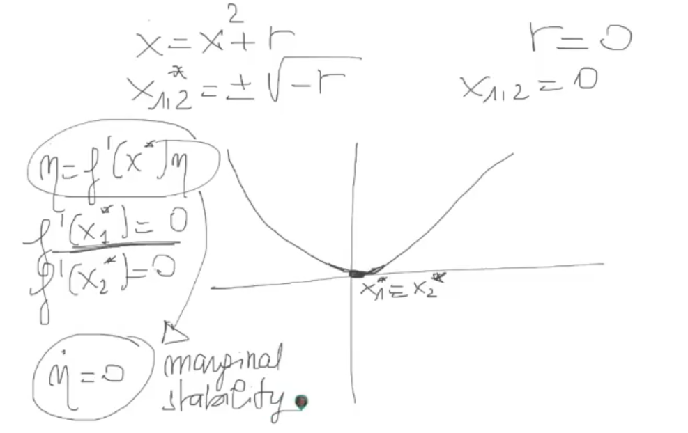
But the actual steady state is NOT!:

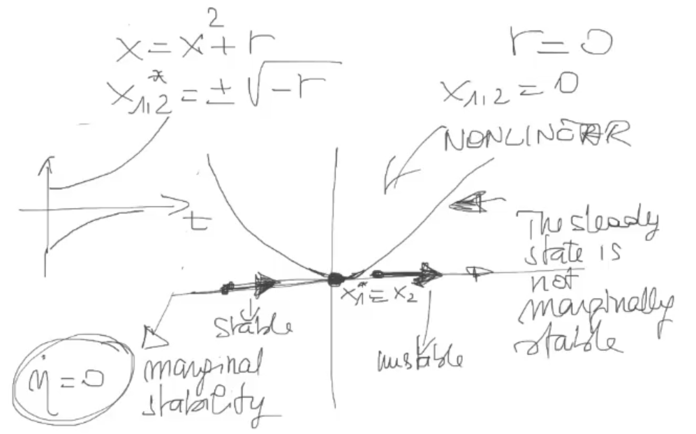
• If we take an inital condition on the left $(x<0)$ than we will have a stable system.
  However it we take an inital condition on the right $(x>0)$ than we will have an unstable system.

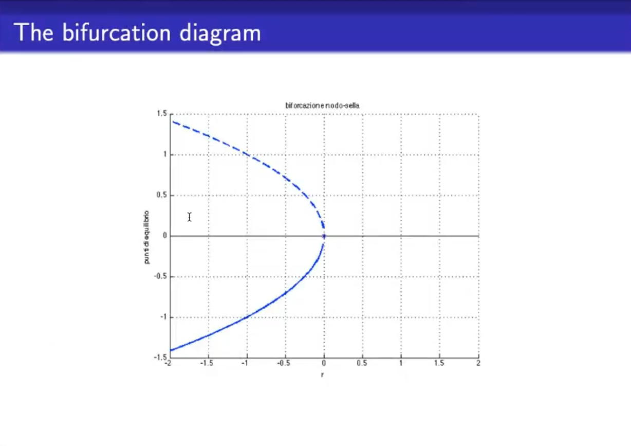
• This is the “bifurcation diagram”.
• The x-axis represents the values of the parameter $r$.
• The y-axis represents the values of the steady states.
• A continuos line represents a stable ss.
• A dotted line represents an unstable ss.
• For $r=0$ we have a bifurcation, and specifically this is a “saddle-node bifurcation”, since we have 1 stable and 1 unstable steady states that collpase.

• This is considered the “simplest case of bifurcation”.
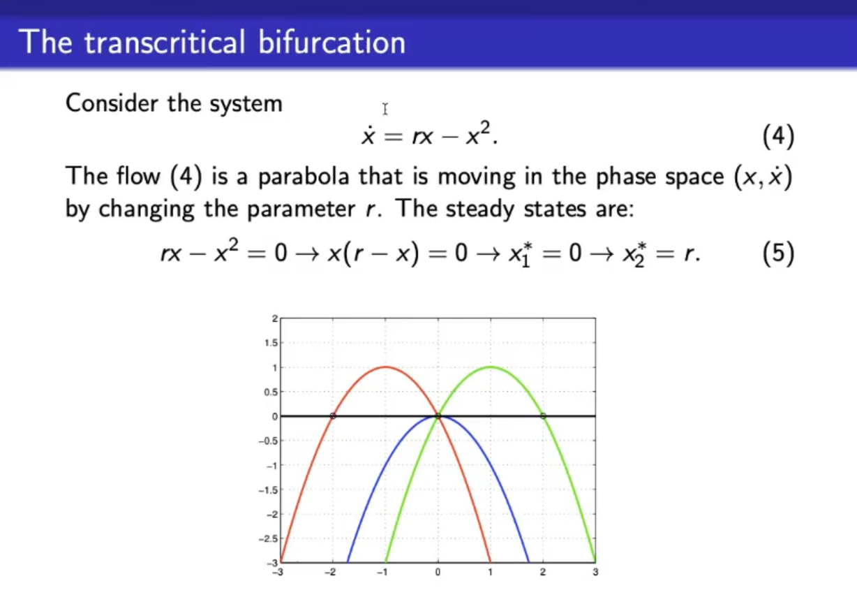
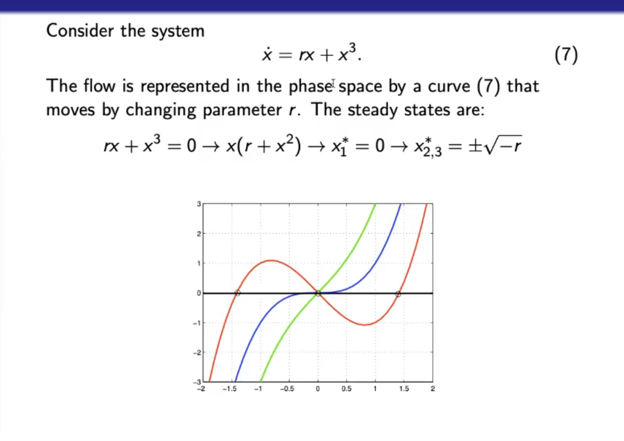
• This system has 2 steady states $x_1^{\ast }=0$ and $x_2^{\ast }=r$.
• Red parabola: $r<0$.
• Green parabola: $r>0$.
• Blue parabola: $r=0$.
• Changin $r$ this time changes the stability of one of the steady states, and differently from before no steady states disappears.

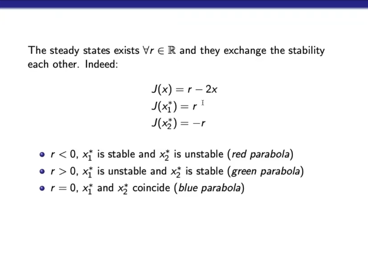
• Analysis of the stability of the steady states.
• Again when the two steady stated conicide for $r=0$ the steady state is stable from on part, and unstable from the other part, like for the saddle-node bifurcation.

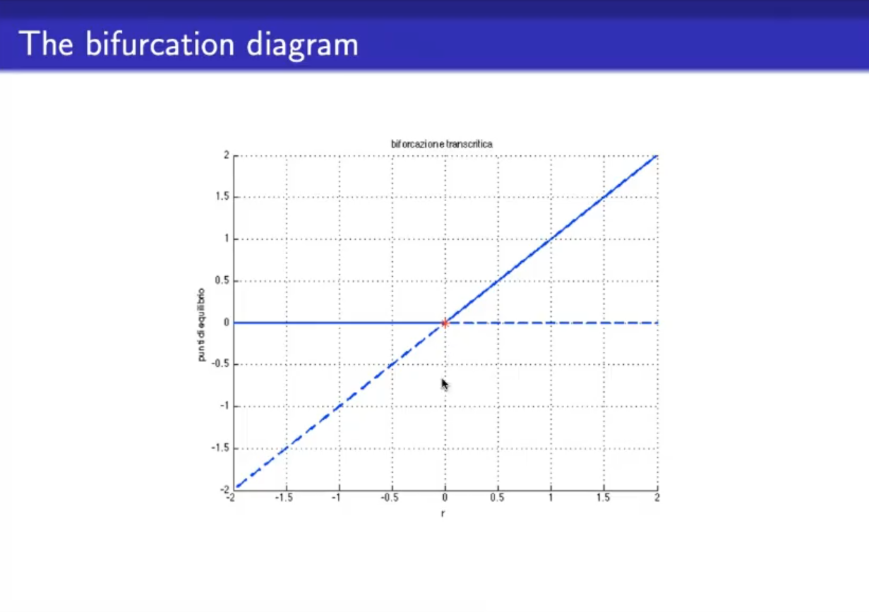
• This is called the “Transcritical Bifurcation”

• The blue curve has a $0$-derivative for $x=0$

Let’s analyze the steady steates. For 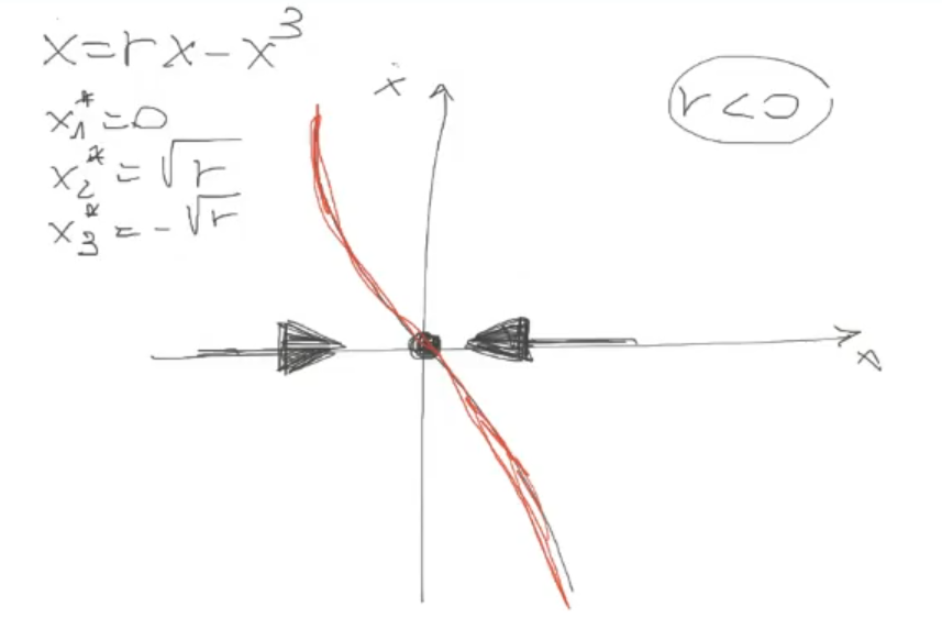$r<0$:
And in case of the blue curve, $r=0$:
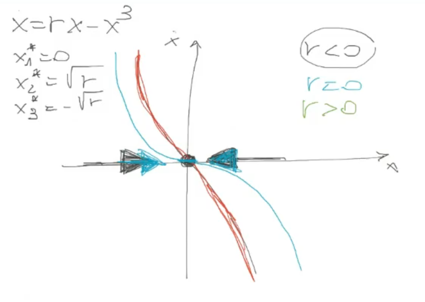While for $r>0$:

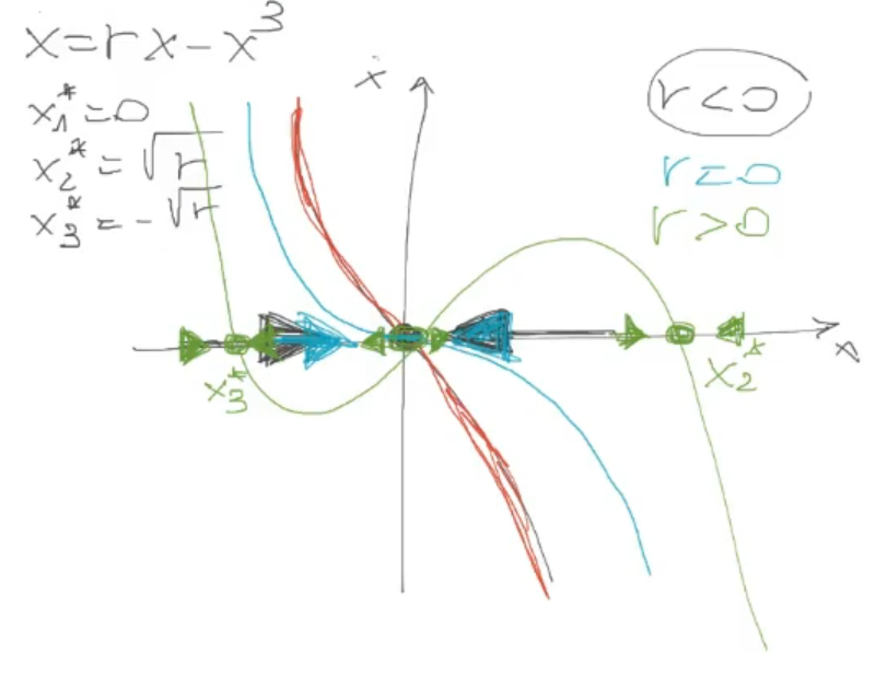
• From the red curve, to the green curve, we have that:
  1. $x_1^{\ast }$ looses stability.
  2. $x_2^{\ast },x_3^{\ast }$ are born, and are stable.
• We say that for $r=0$ is when this change happens.

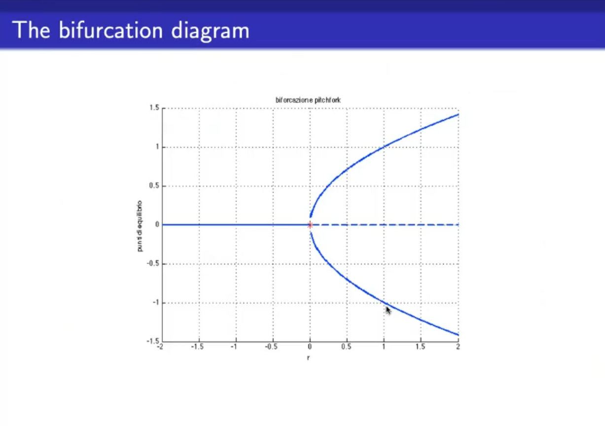
• This is called the “Supercritical Pitchfork Bifurcation”
• We can say that globally this system is stable.

• A similar “sign-switched” case of the previous one.

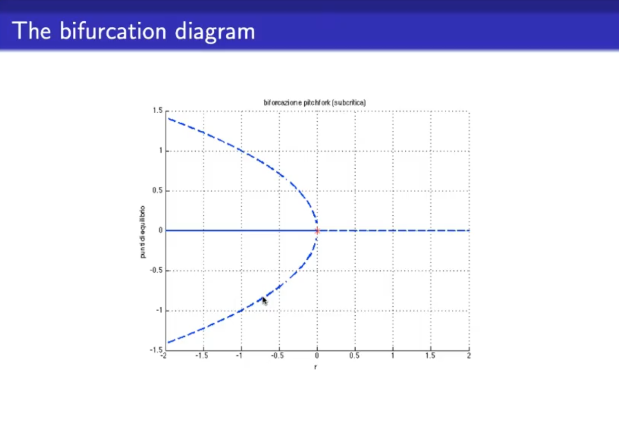
• This is called the “Subcritical Pitchfork Bifurcation”

If we analyze the supercritical pithfork bifurcation, we can see that: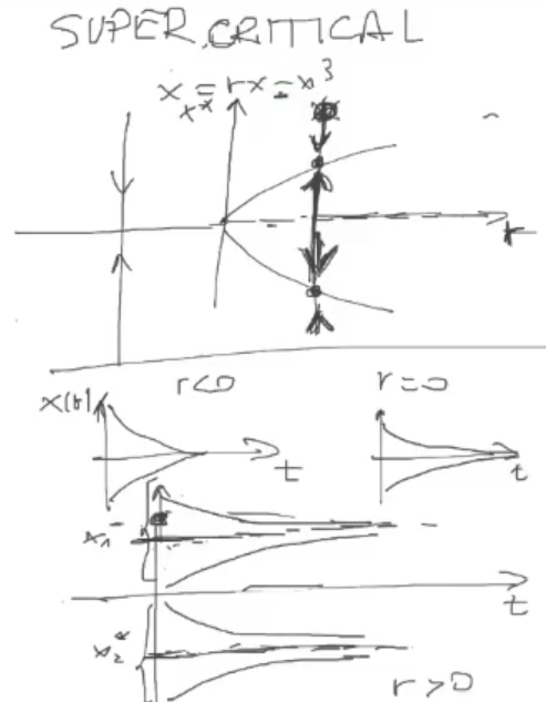

• For whichever value $r$ assumes, the system will converge, except for $x^{\ast }=0,r=0$ for which the system will remain at $0$ (unstable steady state)

While for the subcritical case: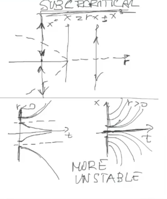

• The system is a lot more unstable.

NOTE: A bifurcation only appers when there is a non-hyperbolic steady state, this is true also for higher dimensions systems.