Remember:
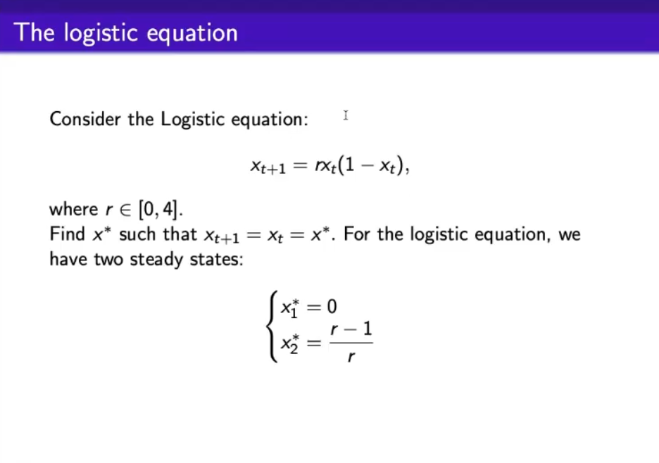
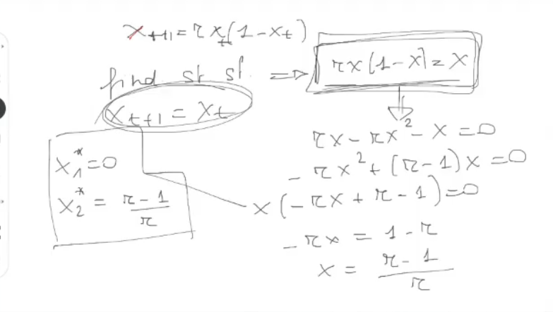
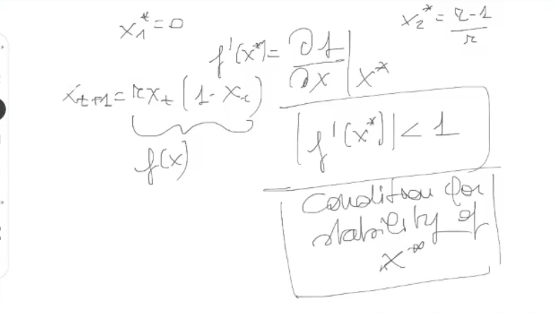
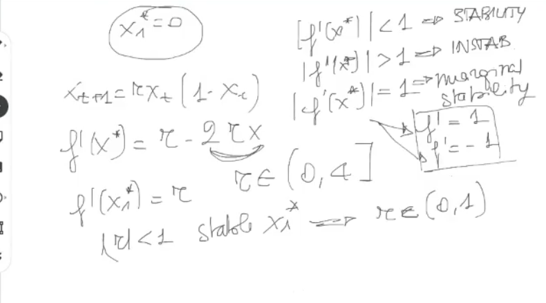
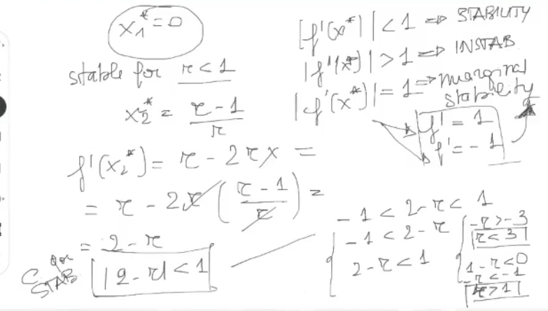
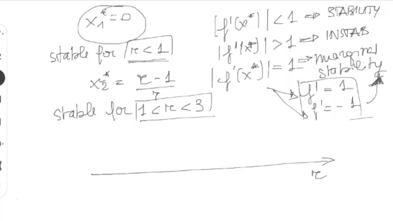
Discrete Time Logistic Equation:Where: , meaning is excluded. If we search for the steady states we will find:
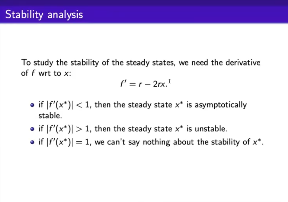
Stability Analysis: To study the stability we need first to calculate the derivative of , so for the logistic equation, with :And from this we can say:
- If : then the steady state is asymptotically stable.
- If : then the steady state is unstable.
- If : then we cannot say anything about the stability of .
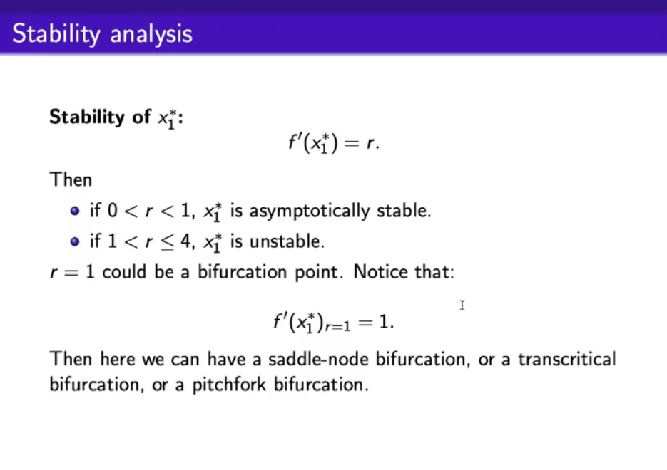
~Ex.: stability of : Then:
- For: : is asymptotically stable.
- For: : is unstable.
- For then we could have a bifurcation point, notice that:For discrete time system the , is equivalent to the continus time case where .
- Then we can have a saddle-node bifurcation, a transcritical bifurcation or a pitchfork bifurcation.
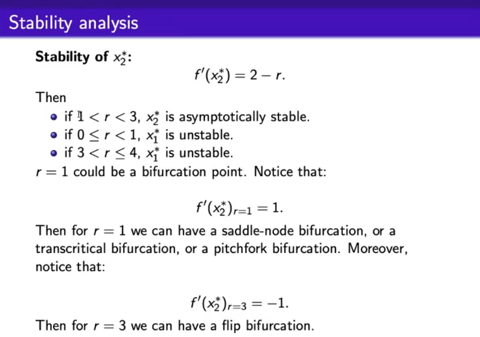
~Ex.: stability of : Then:
- If : is unstable.
- If : is asymptotically stable.
- If : is unstable.
- So for we could have a bifurcation point, since like for the example:Like before, we can have a saddle-node bifurcation, a transcritical bifurcation or a pitchfork bifurcation.
- Also for :We have another bifurcation point, but in this case we have a flip bifurcation, where the flip bifurcation is the equivalent of the hopf bifurcation for discrete time systems.
NOTE: we need to verify that this is in fact a flip bifurcation via simulation.
Here’s the bifurcation diagram:
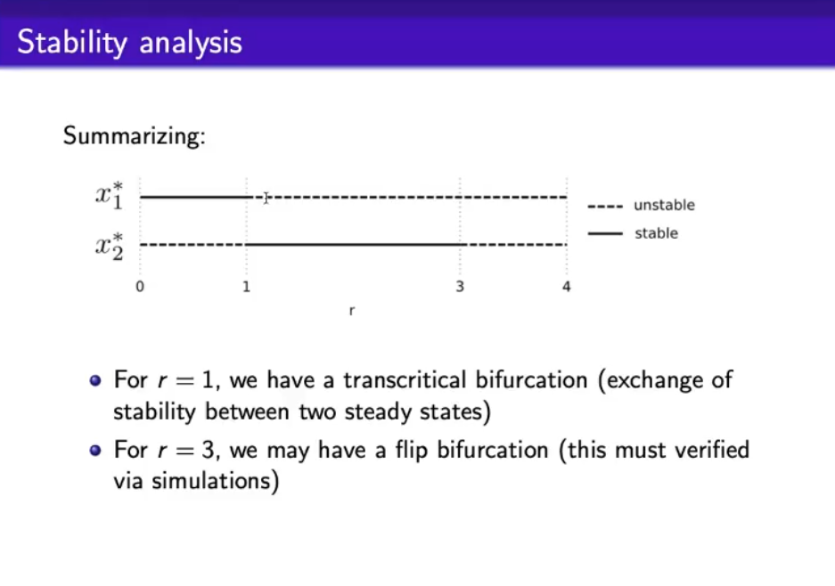
So as a recap we have that:
- , and
- For , we have asympt. stable, and unstable.
- For , we have unstable, and asympt. stable.
- For , we have unstable, and unstable.
- Here’s a drawing to better undestand:
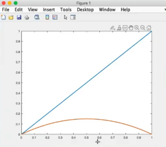
Let’s see the cobweb graph:
- We start by drawing the bisector line (representing ) and the function , and in this case , the logistic funciton.
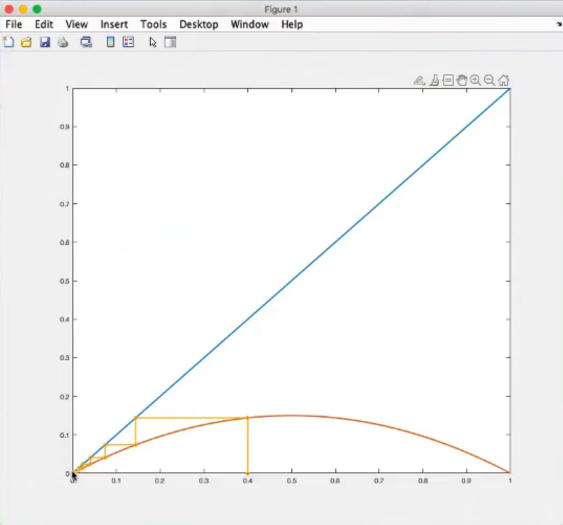
We choose an arbitrary parameter :- We choose an arbitrary initial condition , and start by calculating the next step, meaning :
- We choose the last arbitrary value, the number of steps for drawin the cobweb graph, we have choosen :
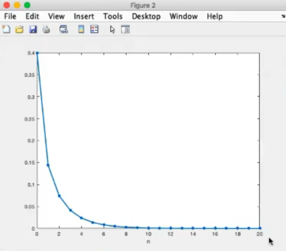
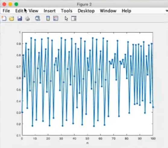
And we iterate: , then and so on…- This confirms that this is an asympotically stable bahaviour, we can also see it by plotting the progession of values, or solution of the discrete time system:
We can change the values: (parameter), (intial conditions) and (number of steps), to see how the system evolves.
logistic_cobweb(r=1.2, x0=0.4, n=20):
logistic_cobweb(r=1.2, x0=0.01, n=20):
logistic_cobweb(r=2.0, x0=0.4, n=20):
logistic_cobweb(r=2.0, x0=0.4, n=20):
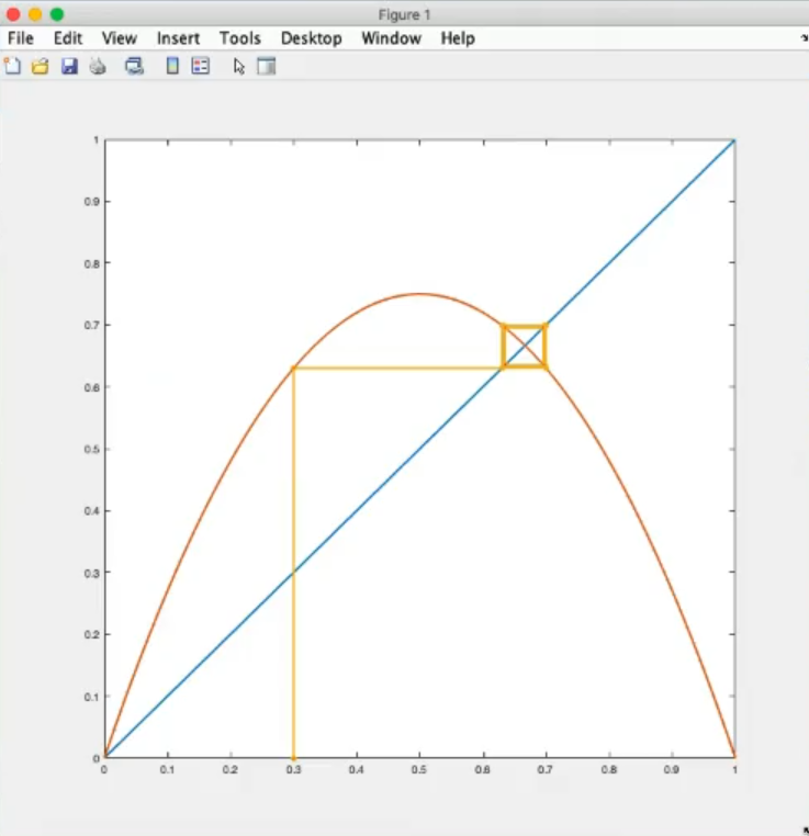
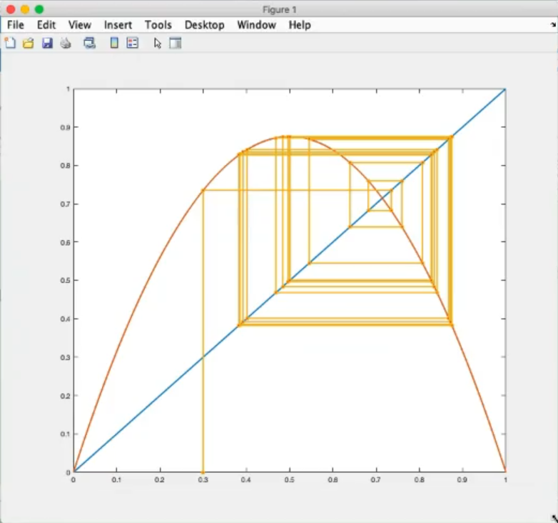
logistic_cobweb(r=2.8, x0=0.3, n=20):
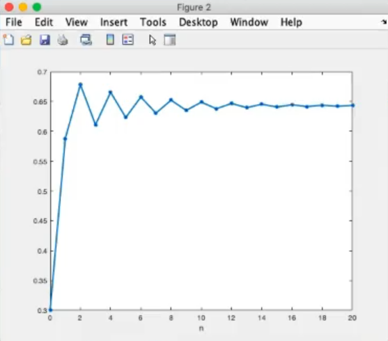
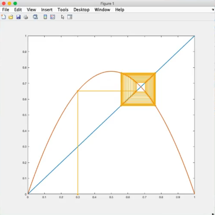
logistic_cobweb(r=3, x0=0.3, n=20):This is called transient dynamic.
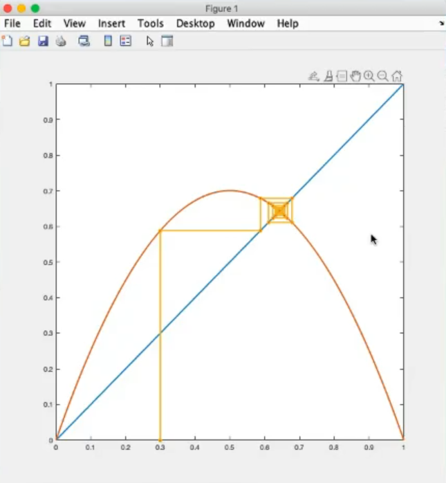
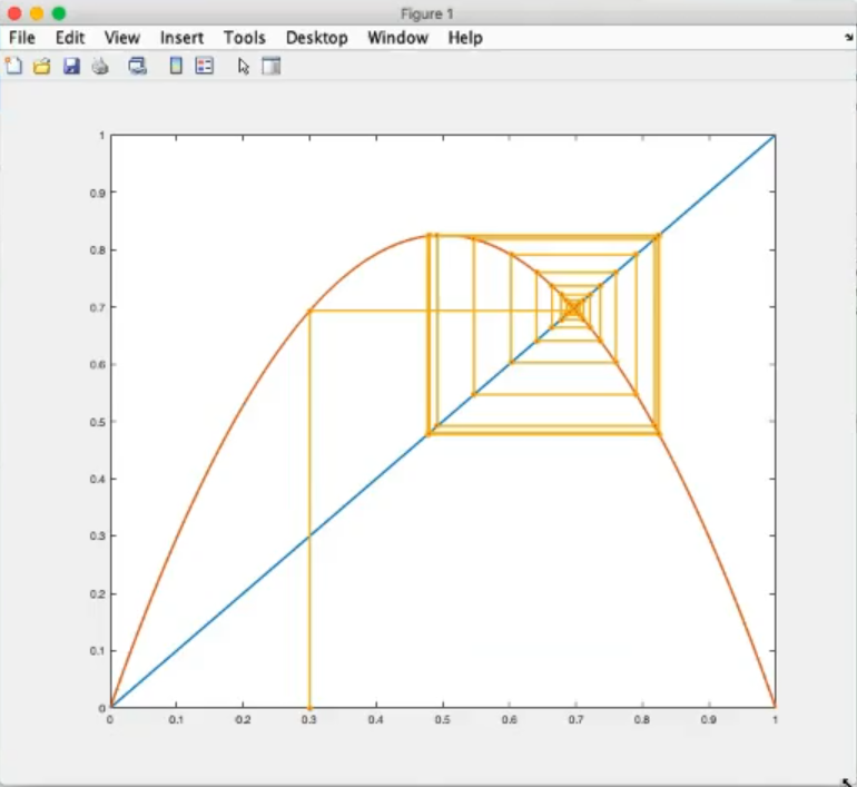
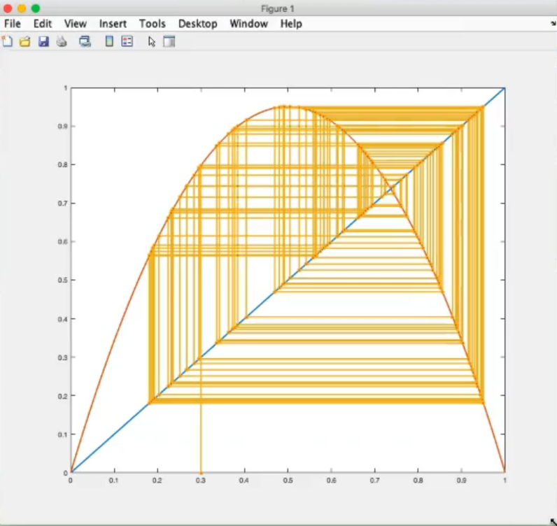
logistic_cobweb(r=3.1, x0=0.3, n=100):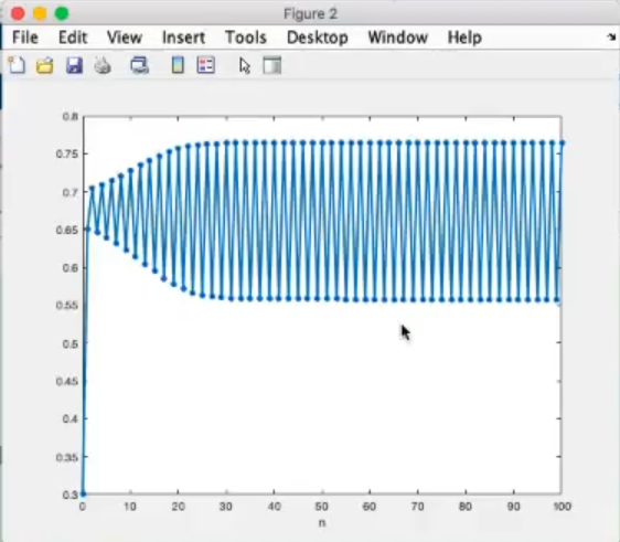
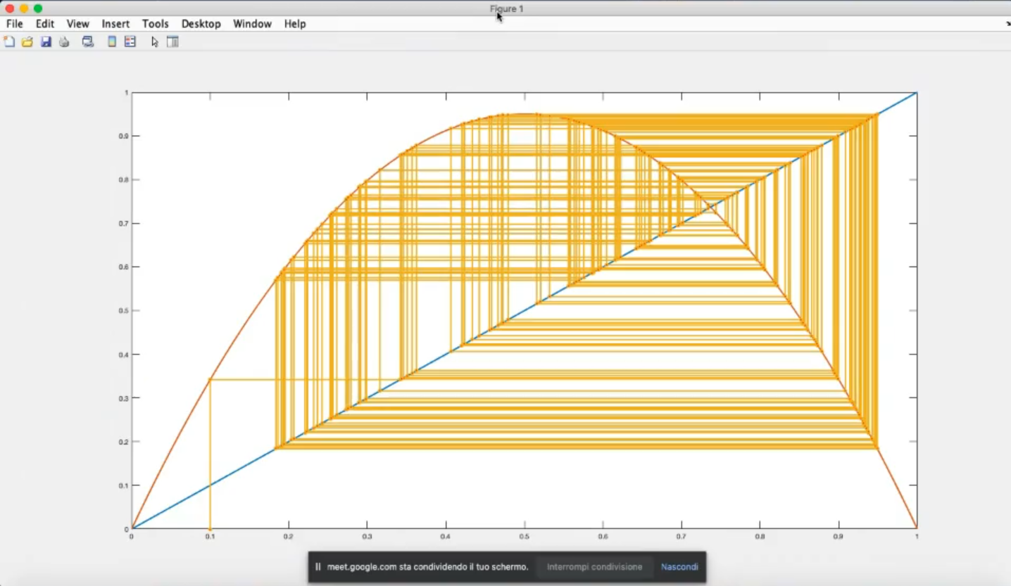
logistic_cobweb(r=3.5, x0=0.3, n=100):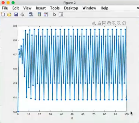
- The trajectory now oscillates beetween points, instead before we could say that it oscillated between points.
- This is the equivalent of the period doubling in the continous time case.
logistic_cobweb(r=3.8, x0=0.3, n=100):
- We have reached the chaotic regime.
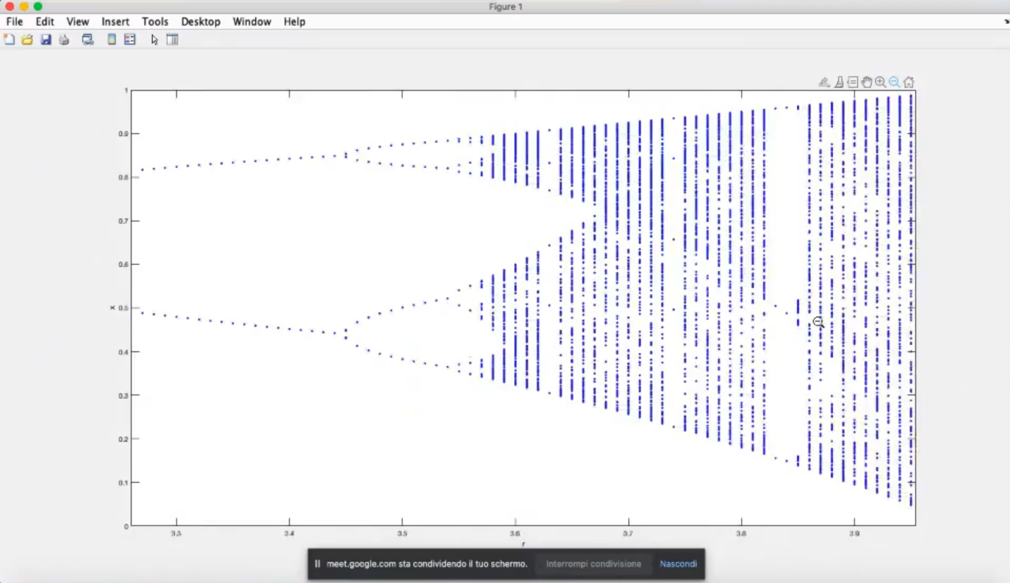
If we draw the bifurcation diagram:
- : the origin is an attractive state.
- : the positive state value begins to rise (the oringin is no longer a stable ss).
- : we have the flip bifurcation, as we have seen in this range we begin exepriencing the first “oscillation” of the system, see this cobweb plot.
- : each of the two branches has its onw flip bifurcation, we have seen it in this cobweb plot we have a period doubling, meaning that instead of having just one oscillation between points, here we have an oscillation between points.
- : one more time, each of the four branches has its onw flip bifurcation.
- Then we have chaos.
- ==As you can see there is a white space in this graph, at about this is the so called “periodic window”==.
Close up of the periodic windows:
- Here we can see that we have periodic windows, we can count the number of “points” in each of them and we can say that:
- The first periodic window at is of period .
- The second periodic window at is of period .
- The first periodic window at is of period .
- There is an error in the slide, it should be , so is excluted.
- is defined as: .
- In discrete case we can have a new type of bifurcation: the “flip bifurcation”.
Some calculations (Lecture 20 - Part 2 @ 11:20 ~ 30:30):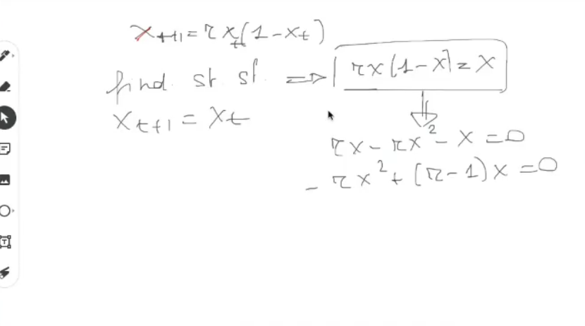
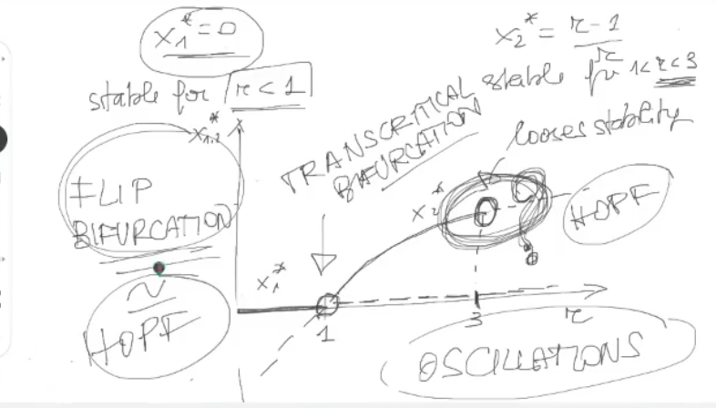
- So the flip bifurcation is the equivalent of the hopf bifurcation for discrete time systems.
- Function
logistic_cobweb(r, x0, n), where:r: parameter .x0: initial conditions.n: number of iterations/steps.
- This are the results for
logistic_cobweb(r=0.6, x0=0.4, n=20)
- Step 1.
- Step 2
- Step 20.
- This confirms that this is an asympotically stable bahaviour.
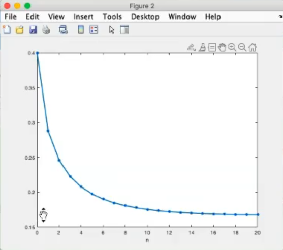
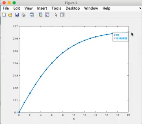
- Progression of values.
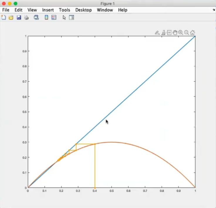
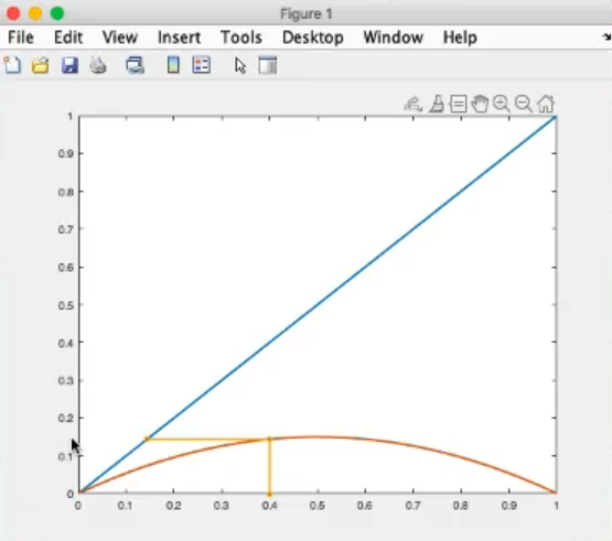
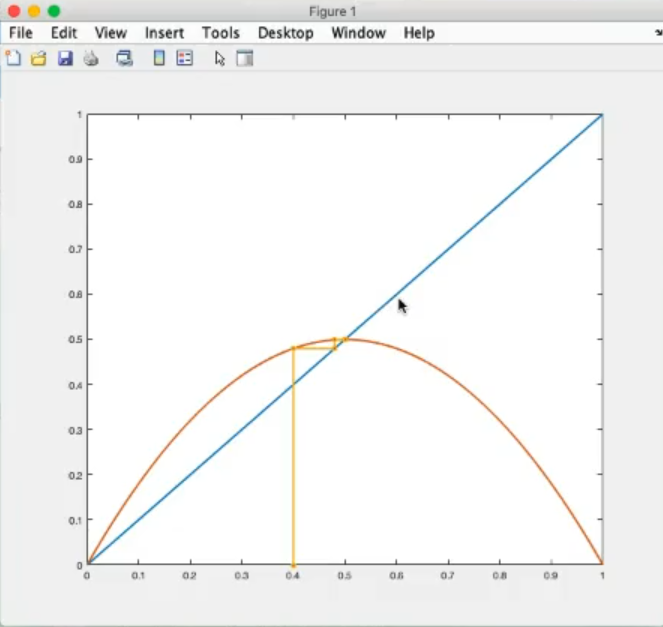
logistic_cobweb(r=1.2, x0=0.4, n=20)- Notice that this time there are two intersections between and the bisector.
- So we have a steady state .
- If we calculate it, it is at .
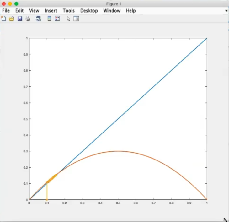
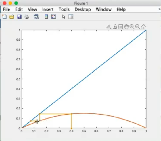
logistic_cobweb(r=1.2, x0=0.1, n=20)
- Again it converges to the same ss as before.
logistic_cobweb(r=2.0, x0=0.4, n=20)- The ss has moved up, and it is still attractive.
logistic_cobweb(r=2.0, x0=0.9, n=20)
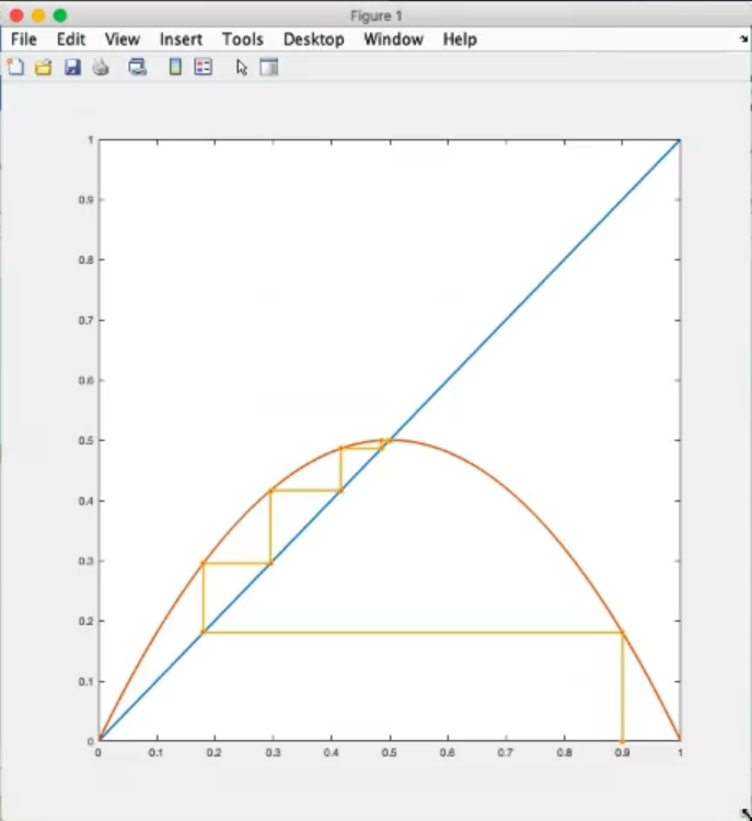
logistic_cobweb(r=2.8, x0=0.3, n=20)
- The system oscillate, but still converges to the ss.
logistic_cobweb(r=3, x0=0.3, n=20)
- Transient dynamic.
logistic_cobweb(r=3.1, x0=0.3, n=100)
logistic_cobweb(r=3.3, x0=0.3, n=100)
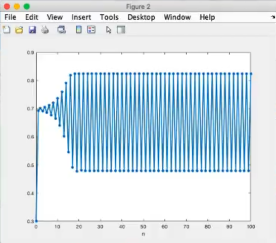
logistic_cobweb(r=3.5, x0=0.3, n=100)- The trajectory now oscillates beetween points, instead before we could say that it oscillated between points.
- This is the equivalent of the period doubling.
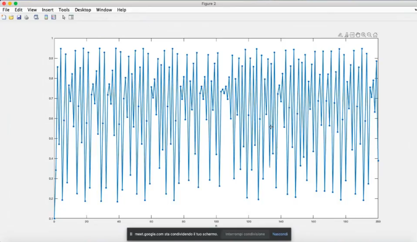
logistic_cobweb(r=3.8, x0=0.3, n=100)
- Chaos
logistic_cobweb(r=3.8, x0=0.1, n=200)- Like for the continous case, we can see that the trajectory will touch every single point in the phase space, without ever assuming the same value twice.
- Lecture 20 - Part 2 @ 53:10 ~ 54:50
- Lecture 20 - Part 2 @ 55:15 ~ 58:51
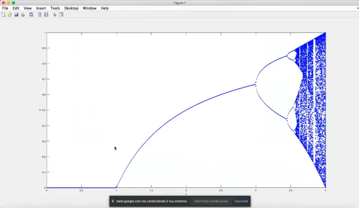
- : the origin is an attractive state.
- : the positive state value begins to rise (the oringin is no longer a stable ss).
- : we have the flip bifurcation, and in the graph we represent the two points of the oscillation.
- : each of the two branches has its onw flip bifurcation.
- : each of the four branches has its onw flip bifurcation.
- Then we have chaos.
- As you can see there is a white space in this graph, at about this is the so called “periodic window”.
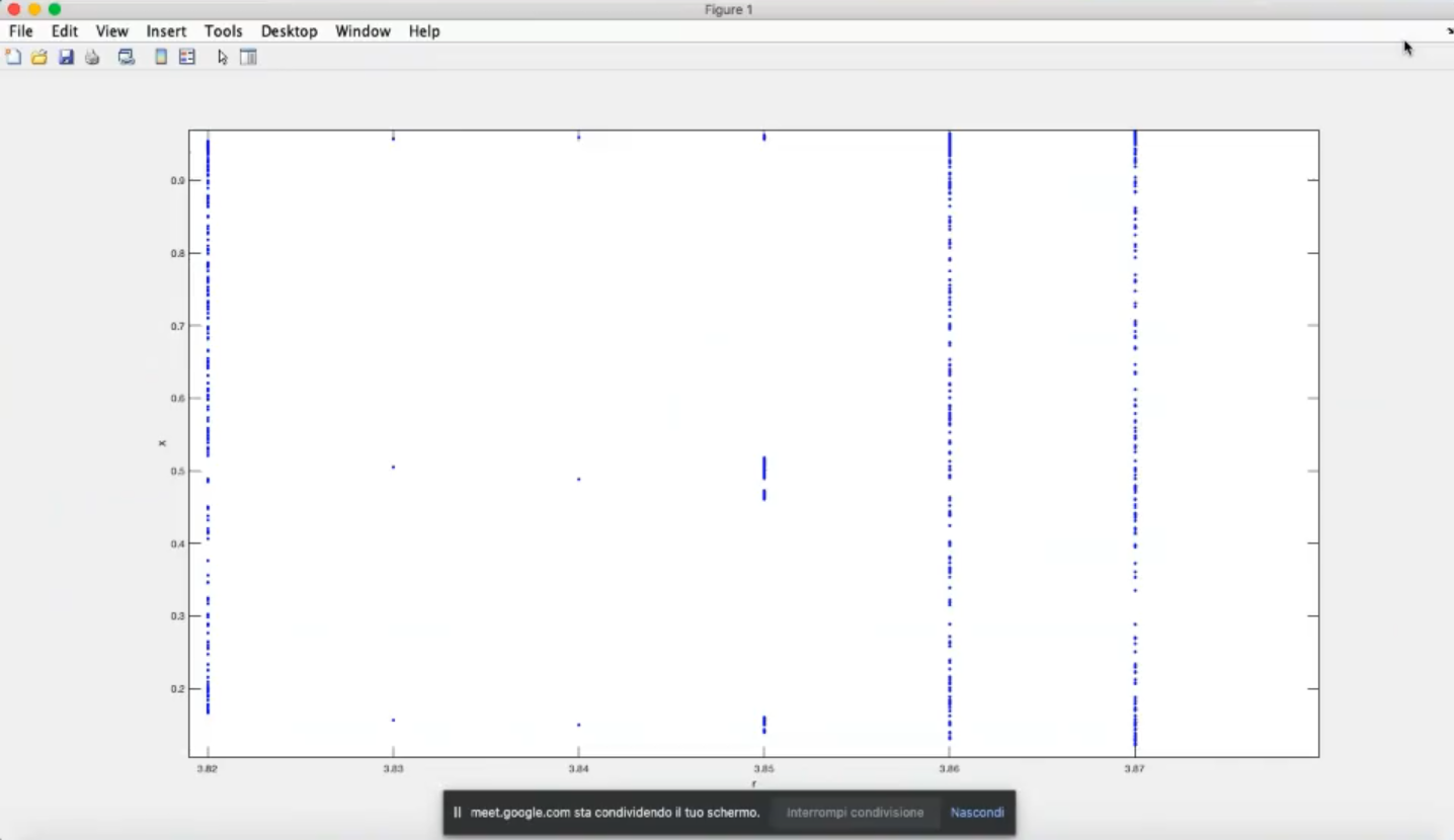
- Close up of the periodic windows.
- Here we can see that we have periodic windows, we can count the number of “points” in each of them and we can say that:
- The first periodic window at is of period .
- The second periodic window at is of period .
- The first periodic window at is of period .