(PNN) Parzen Neural Network
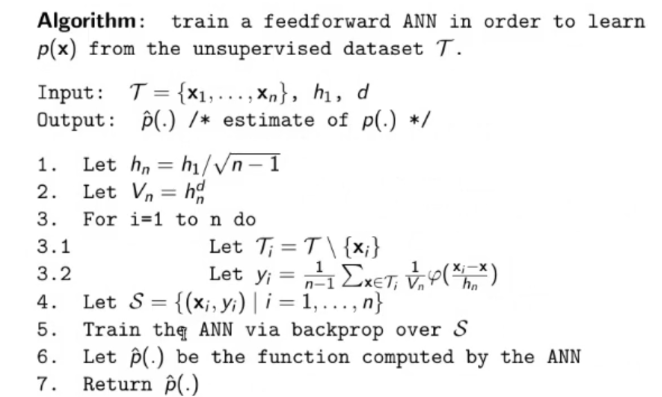
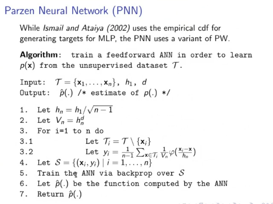
Starting from the training set We want to obtain the estimate of , let’s call it . To do this we can use the following algorithm:
- Define
- Let
- Let
- For
- Let
- Let
- Let a new training set
- Train an ANN via backpropagation over .
- Let be the function computed by the ANN
- Return
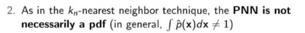
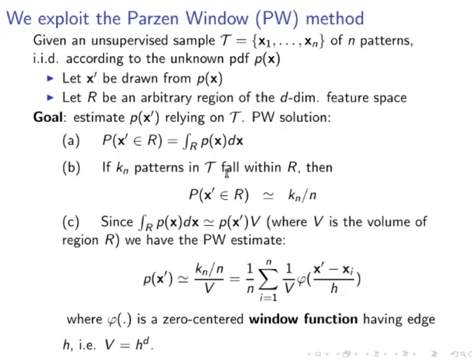
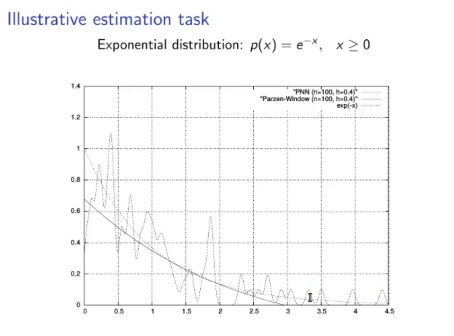
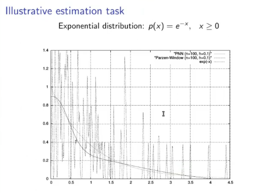
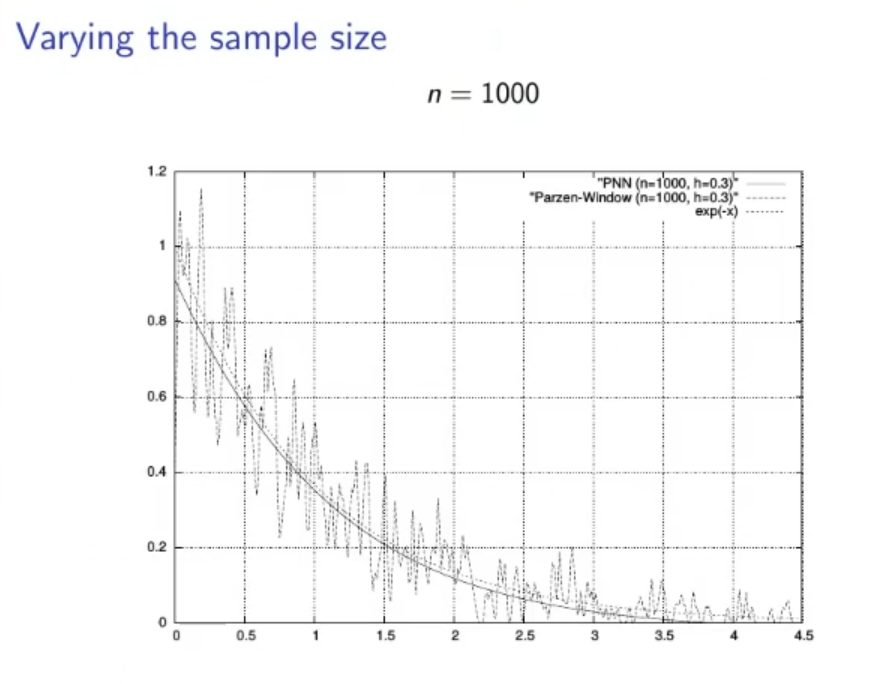
NOTE: is the pdf estimation obtained by the Parzen window
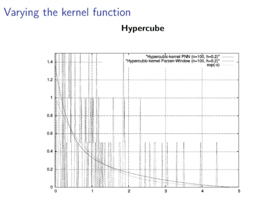
NOTE: is defined as the hypercube function.
Some Insights:
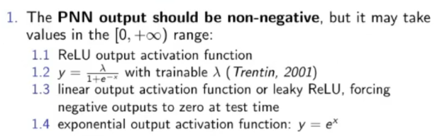
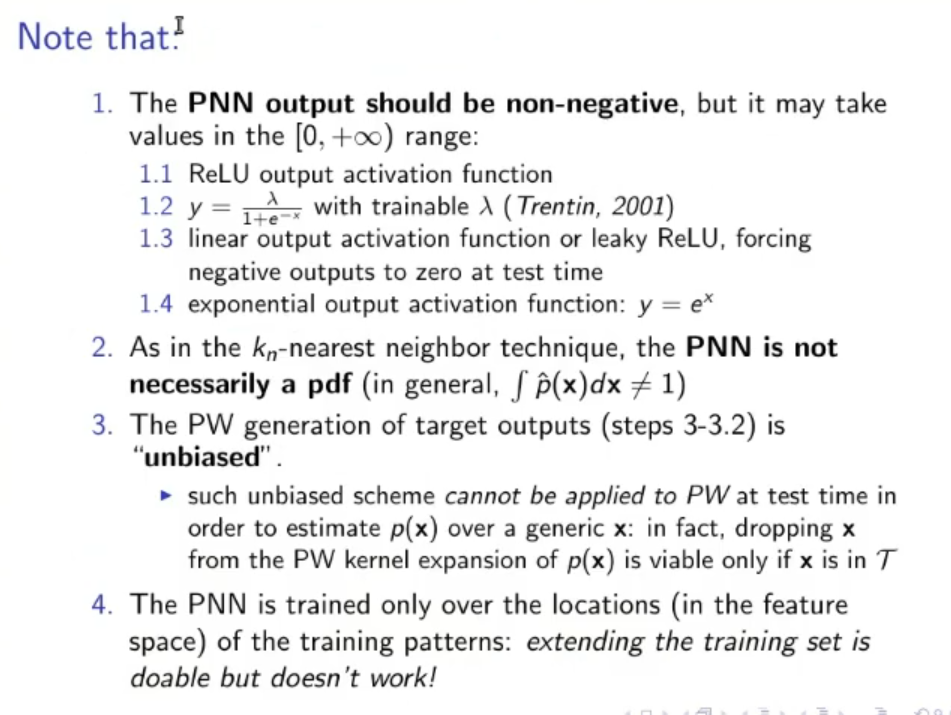
If we use ReLU
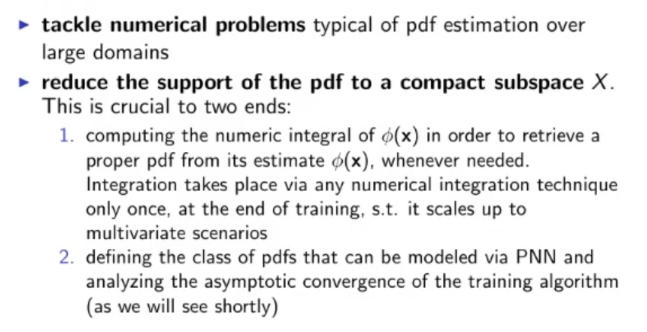
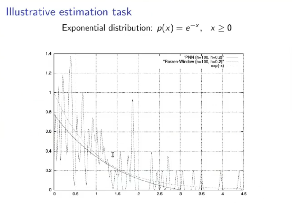
Upgrade of the PNN: Better Approximation of the Tail of the Distribution
- PROBLEM: Using the PNN the output will never reach , this is theoretically correct, but in practice it will result in an error, it’s better to have a PNN that gives when the is really small (an approximation if you will).
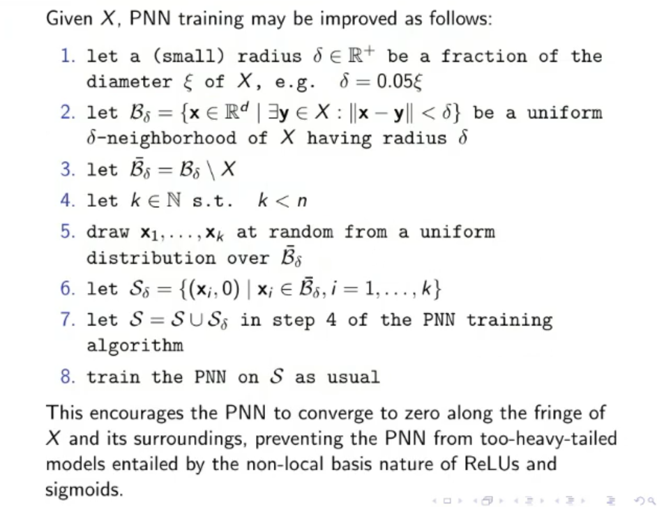
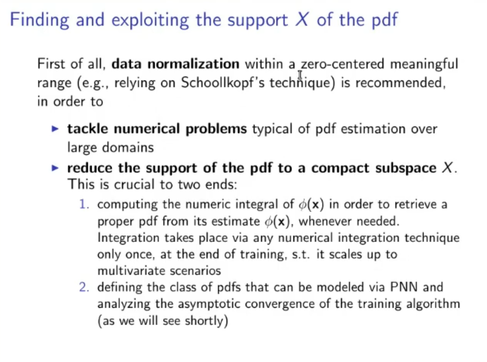
To solve this problem, first we normalize the data (which is always a good practice):
- Let’s choose a meaningful interval zero-centered, for example let’s take .
- We make the data fit into this interval (by normalization).
- We choose some values a little outside
- We add the couples to the training set (the training set to train the ANN) This way we incentive the PNN to actually assume values in the output layer.
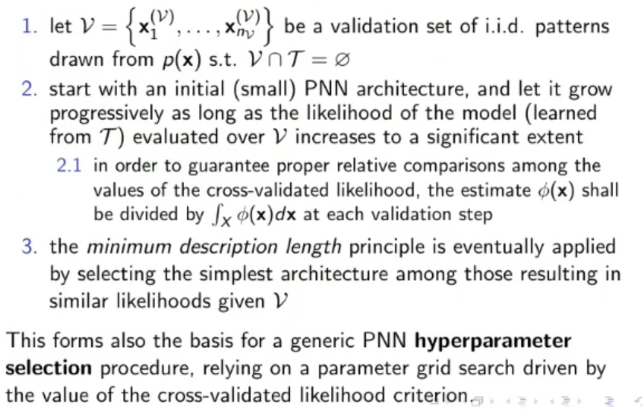
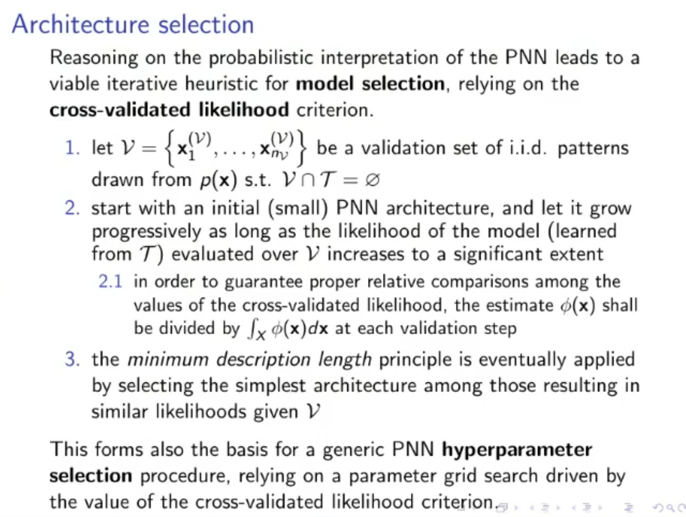
Upgrade of the PNN: Cross-Validated Likelihood
Another upgrade is to separate the training set in a validation set , and another, smaller training set
- Declare (not too big)
- Choose and extract samples from , creating another training set
- Execute the PNN algorithm over
- Evaluate the Likelihood of the model (learned from ) over (this likelihood is called cross-validated likelihood)
- If the likelihood is increased significantantly repeat from step , otherwise return the output of the PNN algorithm.
NOTE: The cross-validated likelihood needs to be divided by at each integration step to be comparable
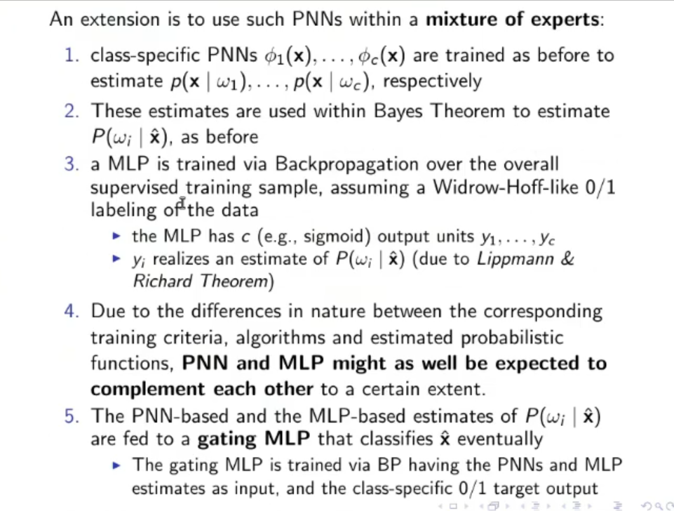
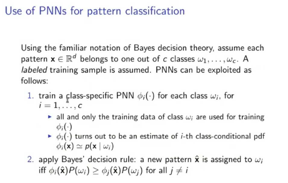
Upgrade of the PNN: Mixture of Experts
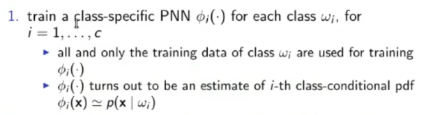
- Create PNNs one for each class for
- Train each PNN only on the data from its respective class
- The output of the -th PNN is the conditional probability
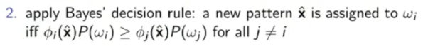
- Now we can apply the Bayes Decision Rule to decide to which class belongs to:
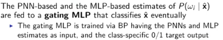
- We consider the PNNs just created a single Expert
- Another one will be:
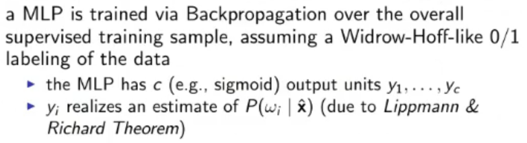 So we have two Expert in parallel now.
 - For the Gather we simply train it using backpropagation
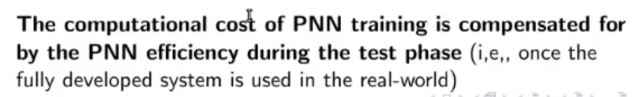
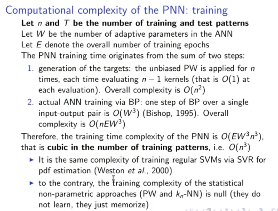
Computational Complexity
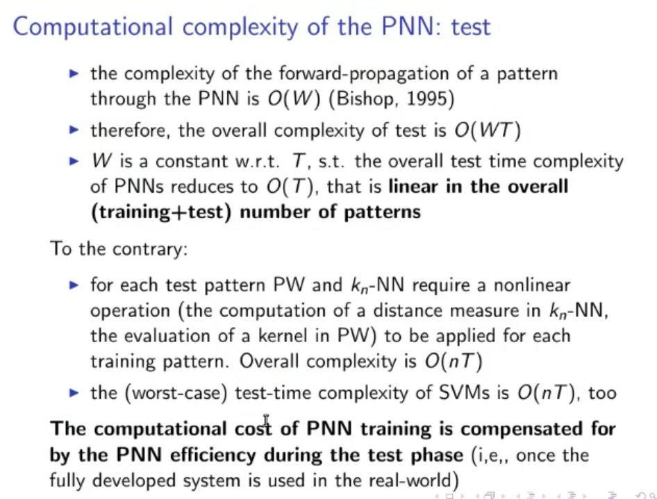
The PNN with respect to the PW takes a long time to train, while the PW requires no training, but once the training is done the PNN requires a miniscule amount of computational complexity to find the estimate, while the PW takes a lot.
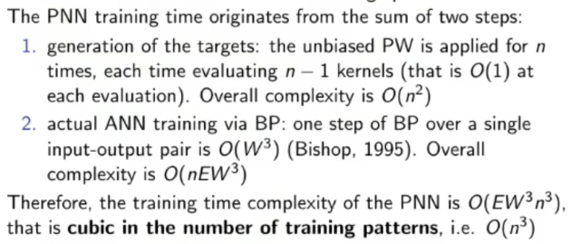
- PNN training:
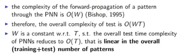
- PNN estimation time:
- PW estimation time:
Nonpaltry PDF
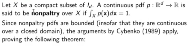
To make it simple a nonpaltry PDF is a PDF that is continuous in expect in a closed subset.
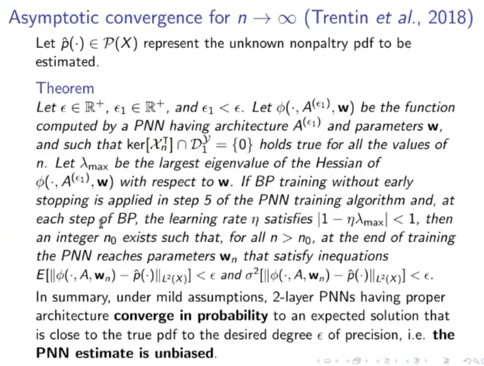
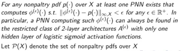
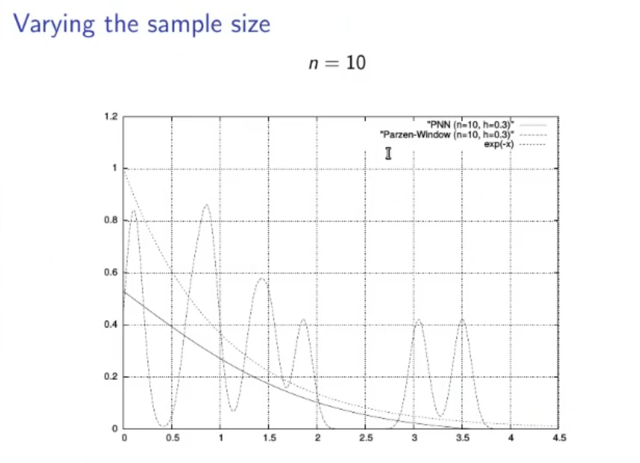
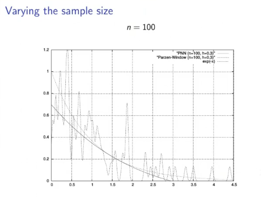
Then for a nonpaltry PDF we have a theorem that says that for the PNN converges to the actual PDF.
From the Slides
Algorithm:
 (The solution listed as are all solution to the problem)
Also in the PNN algorithm it is recommended to normalize data within a zero-centred meaningful range (meaningful range means not too little not to big, to be distinguished from the small zero-center range used in ANN with sigmoid activation function.
This is especially helpful to:
If we know we can upgrade the PNN training algorithm
Architecture Selection
TODO WHAT??
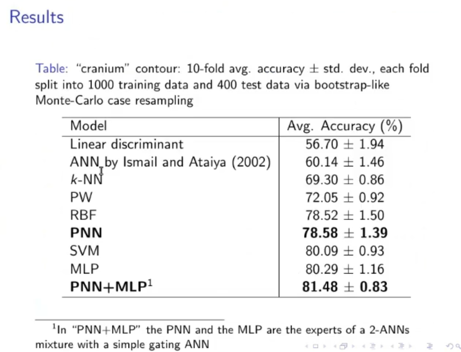
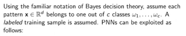
Use of PNNs for pattern classification:
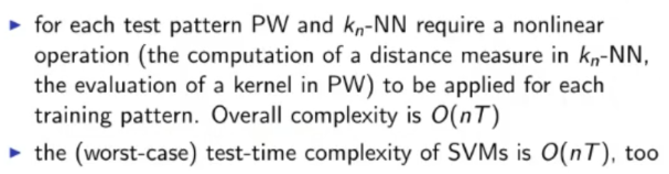
Complexity:
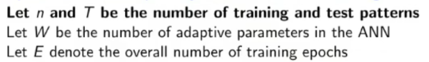
TRAINING COMPLEXITY*:
TEST COMPLEXITY:
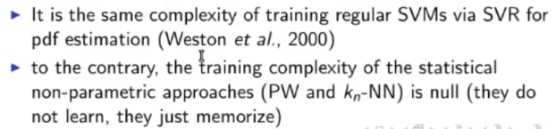
Comparison of training and testing complexity with SVMs (TODO ) and with PW (Parzen Window) and -NN (-Nearest Neighbour)
training comparison
 testing comparison:
 To sum it up:
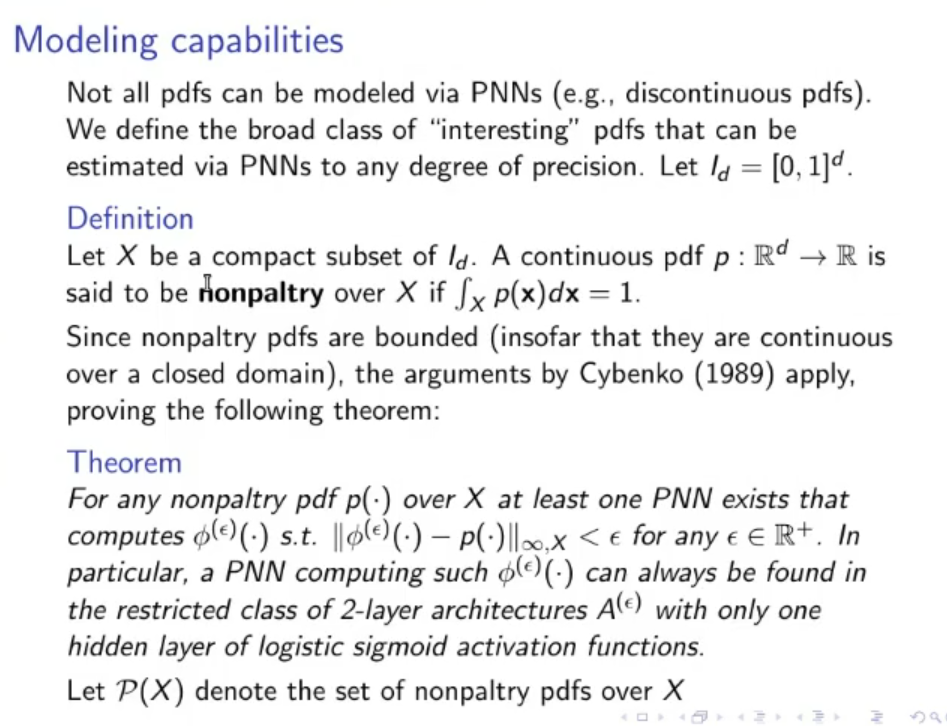
Modelling Capabilities:
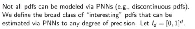
Definition of “Interesting PDFs”:
nonpaltry pdf:
Theorem:
Original Files:
(Not to study):