Turing Machine
Nastro
Alfabeto
Orologio
Testina
Stati Interni
Regole di Transizione
AI Discussion
The Imitation Game
Weak and Strong AI
Classification Problem
Event
Extract Features
Classify
Class
Types of Features
Numeric
Symbolic
Qualitative
Gaussian Distributions
Definition of Gaussian PDF, Multivariate Gaussian PDF, Mean and Variance
Mahalanobis distance
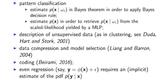
Bayes Theorem
Decision Boundary or Decision Rule
Bayes Decision Rule
Bayes Decision Rule with Discriminant Functions
Maximum Likelihood Decision
Fist Principal Components
Likelihood
Likelihood of given
(ML) Maximum Likelihood Estimate
If we want to find the ML Estimate we need to find such that:
Log-Likelihood
- Instead of the normal we use
- If we want to find the ML Estimate we need to find such that:
Gaussian ML Estimate:
- If the PDF we want to estimate is Gaussian, then the ML Estimate is the Gaussian PDF having mean equal to the sample mean and variance equal to the sample variance.
Validation of Classifiers
Normal Method with 60/20/20 Training Validation Test Sets
“Leave One Out” Method
- Used if the data sample is small and it is difficult/expensive to add data
- For each single data, we iterate, the training set will be data, the validation set will be only piece of data, the error is computed averaging all the error on the validation sets.
- At each iteration changes
“Many-Fold Crossvalidation” Method
- Alternative to the normal method, it is based on the idea of the “Leave One Out” method.
- Scales much better than the “Leave One Out” method.
- Same as “Leave One Out” method, but instead of using piece of data for the Validation set we use data, where of course .
- Like the LOO method, at each iteration changes.
- Each new validation set of size (created at each iteration) has data never used before in previous validation set.
Supervised Learning
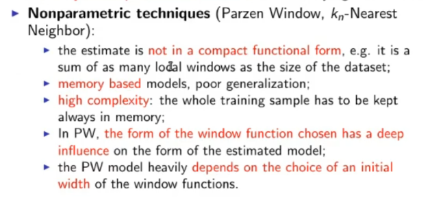
Non-Parametric Estimates
Relative Frequency Estimate
- If out of data are in , we can estimate via the relative frequency:
Easily Estimate a PDF:
~Ex.: we are searching for the pdf of males in a specific university, we use the region to estimate from data.
- The estimate of out of data is defined as: .
Then the estimate will be calculated from:
- be the volume of .
- be the number of data (out of ) in .
⇒ Then, the estimate of will be equal to:
Asymptotic Necessary and Sufficient Conditions
- We want to ensure , so:
- (to guarantee convergence)
Solutions:
- PARZEN WINDOW: Fix the volume (~Ex.: ) and determine consequently.
- -NEAREST NEIGHBOUR: Fix (~Ex.: ), and determine consequently, in such a way that exactly patterns fall in .
K-NN
Parzen Window
Kernels
- Before applying the Parzen Window or K-NN method, we apply a filter to the data using a kernel.
Hypercube Kernel
- The easiest kernel, it result into a steep separation of the data into inside and outside the region
- The kernel formula is:
Gaussian Kernel
- Most useful if the pdf to be estimated is Gaussian
Dirac’s Kernel
- Where is the hypercube kernel function.
- .
- If is big the function is a very smooth function.
- if is really small, , than is a Dirac’s Delta centered in .
- This was used as an useful example to understand how a different kernel can impact the quality of the estimate .
Estimated Probability
- Given a region with center in (which is the data we want to estimate)
- Let’s say we have (labeled) data points inside .
- Let’s also say that we have data points in are labeled as belonging to class
- Then the estimated probability is equal to:
Nearest Neighbour Rule:
- the pattern to be classified will be classified with the nearest labeled data .
- Let’s say belongs to class , then we classify with class
- It’s the same as doing a 1-NN classification
-NN (-Nearest Neighbour)
- Same as K-NN but instead of deciding on an arbitrary at the start, we decide on a which depends on the number of data
- ~Ex.:
- Alpha is an hyperparameter that we can be decided arbitrarily, for example .
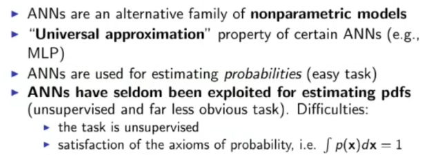
ANN
Architecture
- directed or un-directed graph
- each node (or vertices) is called a neuron and each arch (or edge) is called a synaptic connection
- For each node we can define an activation function
- While for each arch we can define its weight.
- An architecture is completely defined with: Vertices, Edges, Input Units, Output Units, Hidden Units, Weights and Activation Functions.
- Typical Activation function: Sigmoid function:
Dynamics
- Defines “How the signal propagates”.
- Normal Dynamics are: The input data propagates from the input layer up to the output layer passing all hidden layer, every time a set of data propagates to a new layer, the arch that go into a single neuron are multiplied with their respective weights and the summed all together, lastly the activation function of the neuron is applied, this process repeat for each layer up to the output layer.
Training & Generalization
- The ANN learns from the examples contained in the training set.
- We can distinguish between a variety of learning types:
- Supervised: all training data is labeled
- Unsupervised: none of the training data is labeled
- Semi-Supervised: some of the training data is labeled
- Reinforcement: a reinforcement signal (either a penalty or a reward) is given every now and then.
- Learning it’s not enough if we do not generalize, that is, it’s necessary that the model will provide sufficient results when given new data.
MLP (Multilayer Perceptron)
Fully Connected layered architecture with feed-forward propagation of input signals.
- Activation Functions are usually sigmoid and/or linear
- Dynamics: simultaneous propagation of the signal with no delays, from the input layer to the output layer, traversing an arbitrary number of hidden layer (even hidden layers is acceptable)
- Learning: supervised, via the gradient method (backpropagation)
SP (Simple Perceptron)
- 1-Layer ANN (no hidden layer, just input and output layer)
Different Learning Methods
Batch Mode:
- For each epoch the model sees all the data in the training set, then calculates the cost summing all the errors.
On-line Mode:
- For each epoch the cost function considers only one piece of data from the data set.
- Useful if we have a constant influx of new data and we want/need to update the model constantly, for example data taken from a website.
Delta Rule
- Once we have calculate the Cost during training, we need to update the weights.
- Using the gradient descent method:
- Instead of calculating every time the derivative of ,we can apply the “delta rule”:
Where:
Practical Insight for training ANN
Randomly initialize weights in a small 0-centered interval
Normalize the Inputs
Regularization: reduce the number of dimension of the data
Weight sharing: reduce the number of weights making two or more synapses use the same weights
Weight-Decay: Numerically smaller weights are usually better, add the sum of all weights to the cost function
Use more flexible activation function
Add a momentum or inertia term
Where: is the momentum rate, how much should we consider the old in the new one.
Main Supervised Learning Tasks
A supervised MLP learns a transformation
- Function approximation: .
- Regression (linear or non-linear) : , where is the multivariate gaussian noise.
- Pattern classification: .
Universality of MLP:
- A non-linear MLP is very flexible
- According tho the theorem of Universality of MLP, an MLP with a hidden layer of sigmoid function an and a linear output is a universal machine.
Mixtures of Experts
- A neural module can also be called an Expert.
- A neural module or expert realizes a function.
- Then a Gather assigns credit to each expert (how much a neural module is reliable), result in the final equation:
Where: is the credit assigned from the Gather
Divide et Conquer
- The feature region may be partitioned and each partition given to a different expert, usually when used this approach the gather will give a credit of to only one expert at a time (the one that knows about the current region) and all the the other credits will be equal to .
Overlapping regions
- Each expert will express a “likelihood” of being competent over any input , the gather will assign credits according to a pdf under the condition that and imposed during both training and test.
Training the whole Mixture of Experts
- Instead of training each expert separately, we can train the whole model including the Gather, which can learn automatically the values of all credits ()
- The Expert and the Gather are trained in parallel.
Autoencoder
An ANN where the training data is defined as
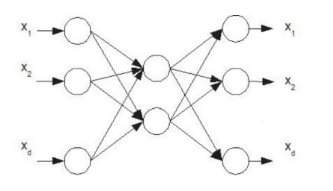
Uses of an Autoencoder
- Let be the original feature space, , so our goal is to train an ANN to realize the function .
- From we define the training set for our autoencoder: and then train our autoencoder.
- We remove just the output layer from our autoencoder and obtain a new function such that , using this function on the input we obtain a new set
- We train a new MLP via backpropagation on and we obtain the function .
- We mount the two MLP (autoencoder and new MLP) on top of each other and obtain the function
- We can tune the completed MLP via backpropagation on the original data set , if necessary
- We can iterate this process stacking even more autoencoder at the beginning of the whole MLP
Using an ANN as a Non-parametric Estimator
- We can use an MLP as a non-parametric estimator for pattern recognition in 2 ways:
- Use MLPs as discriminant function: Train them via backpropagation on a set labeled with outputs.
- Probabilistic interpretation of the MLPs outputs.
- Since the output of an MLP can be seen as:
- We can write:
Which is knows as scaled likelihood.
- is unknown, but can be estimated.
- Also estimates are more robust than estimates, because we need to estimate only one estimate instead of other PDFs ( : number of classes, ), also with the same logic if we estimate only we will have times more data.
- Also if changes over time (let’s say it assumes the new value ) , we can just reuse the same MLP, so no re-training necessary and use the following formula:
Theorem: Lippmann, Richard
- If we reach the global minimum using targets and the right MLP architecture, we are guaranteed that the MLP obtained this way is the optimal Bayesian Classifier, as long as the class-posteriors are continuous.
- In practice, using backpropagation on real world data we will never find the global minimum.
RBF (Radial Basis Function) Networks: A generalized linear discriminant
- All weights between the input layer and the first hidden layer are equal to .
- The RB Function (Radial Basis Function), or kernel is defined as:
- For the learning part, it’s supervised, And we usually consider 2 approaches:
- Via gradient descent over , we learn the parameters: , , and .
- and are estimated statistically, then the other parameters and are estimated via linear algebra methods (such as matrix inversion), or via the precedent method gradient descent.
- Like MLPs, RBF Networks are “universal” approximators.
NOTE: With RBF Networks we can apply gradient-ASCENT over ML (Maximum Likelihood) method in order to estimate PDFs.
The ML method only works if the weights between the last hidden layer and the output layer sum up to .
This can’t be done in MLPs because the constraint is violated, since they realize MLPs realize mixtures of activation functions that are not inherently pdfs.
ML Estimate:
~Ex.: We say that the pdf we want to try is a linear combination of 5 Gaussian PDFs, then we will search such that our assumption will be as close as possible to the real pdf (we minimize the cost)
- We will have that has to respect:
GMM (Gaussian Mixture Model)
k-Means Clustering Algorithm
- Fix initial arbitrary (~ex.: random) values: .
- Assign each (for ) to its closest mean .
- Re-calculate for applying the previous equation for updating (arithmetic mean of the pattern in cluster ).
- If then iterate from point 2., this mean: If during the last iteration at least one value of changed, repeat.
The Problem of Data Description
and are sufficient statistics (they are a complete description of our data) if and only if, our data is drawn from a Gaussian Distribution.
Otherwise they would yield a wrong data description.
To solve this problem we can use a GMM (Gaussian Mixture Model), and relying an an unbounded number of Gaussian Distribution we can describe any continuous and limited PDF. This raises two problems:
- Using an “unbounded” number of Gaussian PDFs brings complexity issues
- Also if we mix too many Gaussian PDFs the problem overfits the training data and doesn’t generalize too well.
Alternatively we can use a non-parametric technique for estimating , for example the Parzen-Window or -Nearest Neighbors, but we need to pay attention to the number of data used:
- If is small (few data), then the estimate is not reliable.
- If is big, then is over-complex, being memory-based, since must be kept in memory and involved in the calculations, this would not be a real data description.
⇒ ==Our best shot is to use Clustering algorithms.==
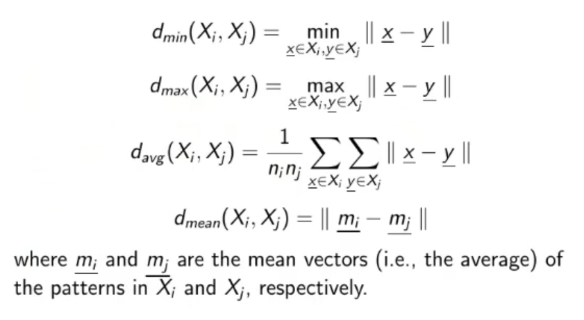
Similarity Measures
- Within Cluster Distance
- Between Cluster Distance

Hierarchical Clustering
Divisive Clustering
- Top-Bottom: Divisive Clustering (we start with 1 big cluster and separate until we have at least or clusters)
Agglomerative Clustering
- Bottom-Up: Agglomerative Clustering, that we will see later (we start with no cluster and agglomerate data into new and previously created cluster until we at least have clusters)
Differences of K-NN Classifier and K-Mean Clustering:
- K-NN is a Supervised machine learning while K-means is an Unsupervised machine learning.
- K-NN is a classification or regression machine learning algorithm while K-means is a clustering machine learning algorithm.
- K-NN is a lazy learner while K-Means is an eager learner. An eager learner has a model fitting that means a training step but a lazy learner does not have a training phase.
- K-NN performs much better if all of the data have the same scale but this is not true for K-means.
Utility of Clustering Algorithms
- Finding the geometric/probabilistic properties of the data: (~ex.: center of mass and variance)
- Describe the data in a concise fashion
- Partitioning the data into sub-samples (useful for dived et conquer algorithms)
- Finding good initialization (the centroids) for complex models such as: GMMs with Max Likelihood, RBFs,
- Discretization of continuous features (~ex.: We can use the centroids and the number of data in each cluster to create an histograms of the data).
- Replacing original big data set with one single cluster of it, useful when working with complex algorithms like K-NN or Parzen-Window.
CNN (Competitive Neural Networks)
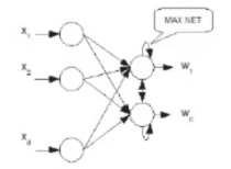 ARCHITECTURE: In the output layer, there are 2 more type of connections:
- Lateral connection (each output neuron is connected to each other output)
- Self-connections (each output neuron has a connection that goes from itself to itself)
The lateral connections are inhibitory (their weights are ) While the self-connections are excitatory (their weights are )
Also at the end of the network there is a MAXNET component that realizes a winner takes all strategy, only one of the output units (a cluster) wins over the others (the losers are set to ).
DYNAMICS: Simple dynamics, the input is passed to the network, the network spits out the outputs ( for ) then the MAXNET selects the winner and turn off all the other outputs.
LEARNING: On-line learning that relies on the following rule:
NOTE: This formula is “theoretically grounded”. Ergo “It’s a good learning formula, we don’t need to search for another one”
Density Estimation:
==MEANING of “Density Estimation” : Estimating PDFs from Unlabeled Data==
Drawbacks of Statistical Approaches
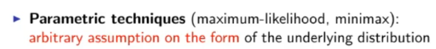
Parametric vs. Non-parametric techniques
Universal Approximator
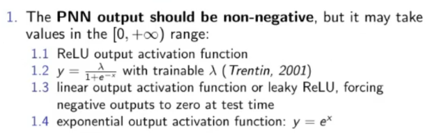
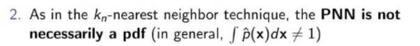
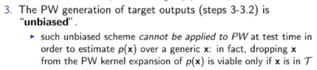
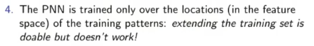
***(PNN) Parzen Neural Network***: ![[Pasted image 20220907163758.png]]
Possible Problems
Symbolic AI: Problem Solving
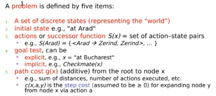

Tree search
- Breadth-first search
- Uniform-cost search
- Depth-first search
- Depth-limited search
- Iterative Deepening search
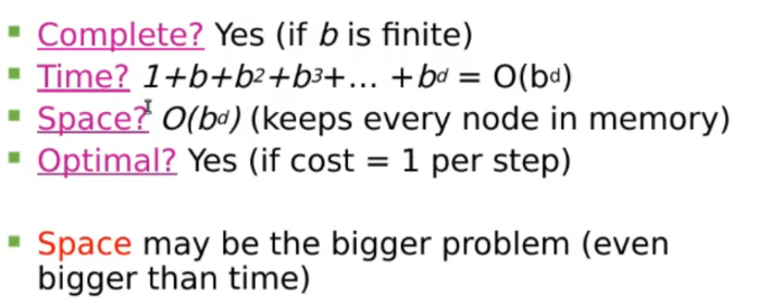
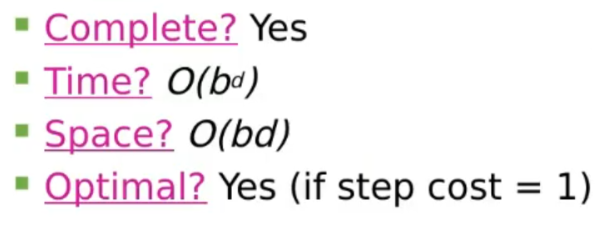
Breadth-first search
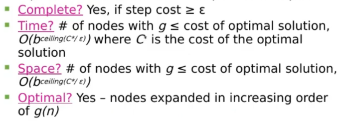
Uniform-Cost Search
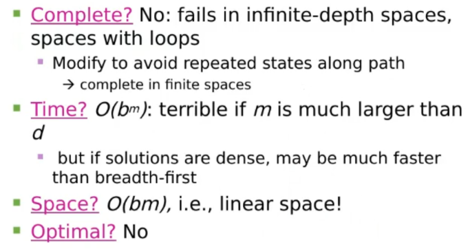
Depth-First Search
(DLS) Depth-Limited Search
Iterative Deepening search
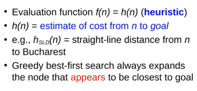
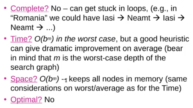
Greedy best-first search
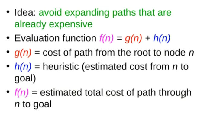
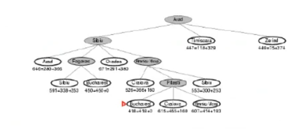
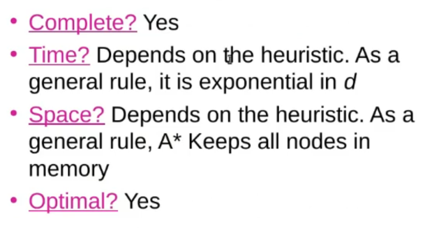
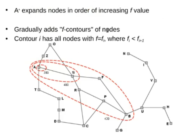
A* Search
Same as Greed-First Search, but also consider the whole cost of the path (from root to node )
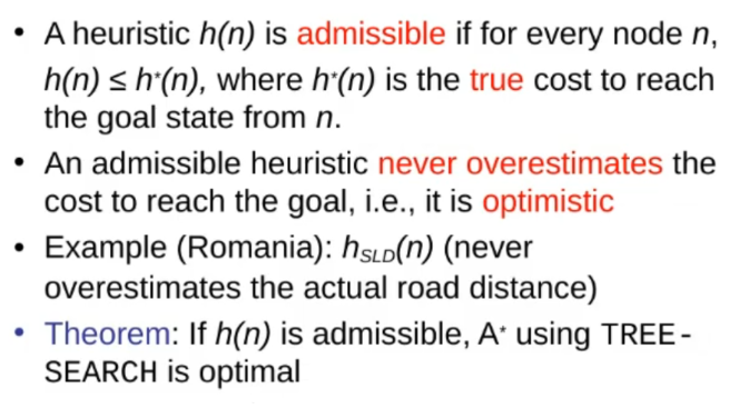
Admissible Heuristic (Definition & Theorem)
Optimality of A* (proof)
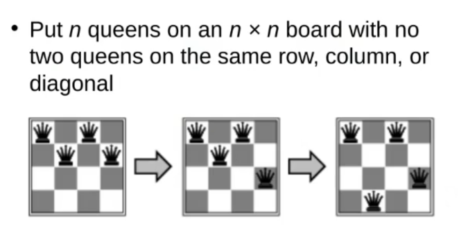
~Ex.: -Queens
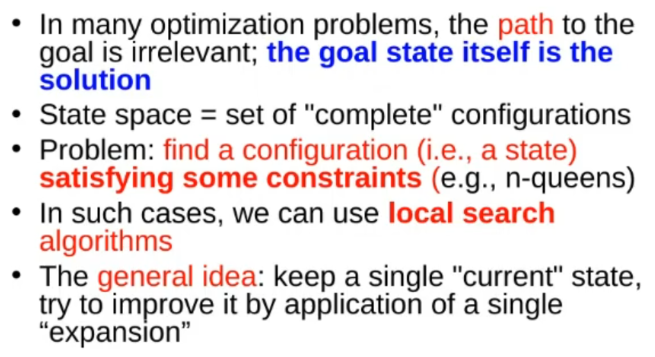
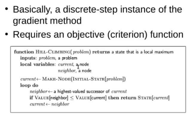
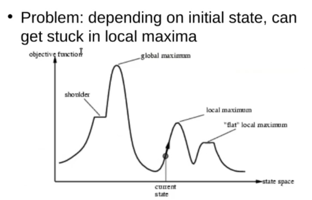
Hill-Climbing Search
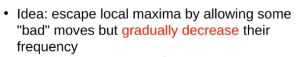
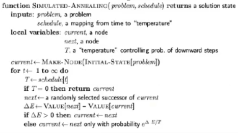
Simulated Annealing Search:
Algorithm:
THEOREM*:
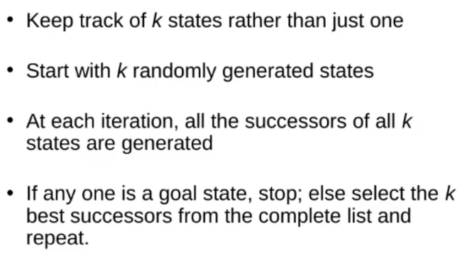
Local Beam Search
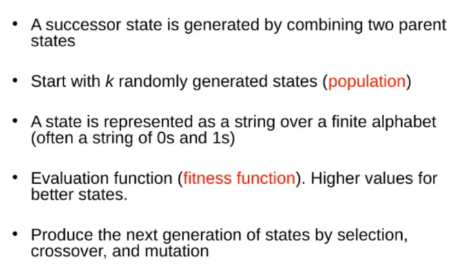
Genetic Algorithms