AI - Lecture 11

Fast Recap:

• ANN (Artificial Neural Network)
  1. Architecture
  2. Dynamics
  3. Training & Generalization
• MLP (Multilayer Perceptron)
• SP (Simple Perceptron)
• Learning Methods for ANN
  • Batch Mode
  • On-Line Mode

---

Recap:

$k_n$-NN ($k_n$-Nearest Neighbour) Decision Rule:

1. Define, $\underline{x_0}$ the pattern to be classified.
2. Create an hypersphere of dimension $d$ around $\underline{x_0}$.
3. Let the sphere expand until it includes $k_n=\sqrt{n}$ data, where $n$ is the total number of data (training, validation and testing).
4. Calculate the volume $V_n$ of this hypersphere.
5. $p_n(\underline{x_0})=\frac{k_n}{n{V}_n}=\frac{1}{\sqrt{n}{V}_n}$

NOTE: To have more flexibility we can define $k_n=\alpha \cdot \sqrt{n}$ where $\alpha \in \mathbb{R}$ is an hyperparameter decided arbitrarily.

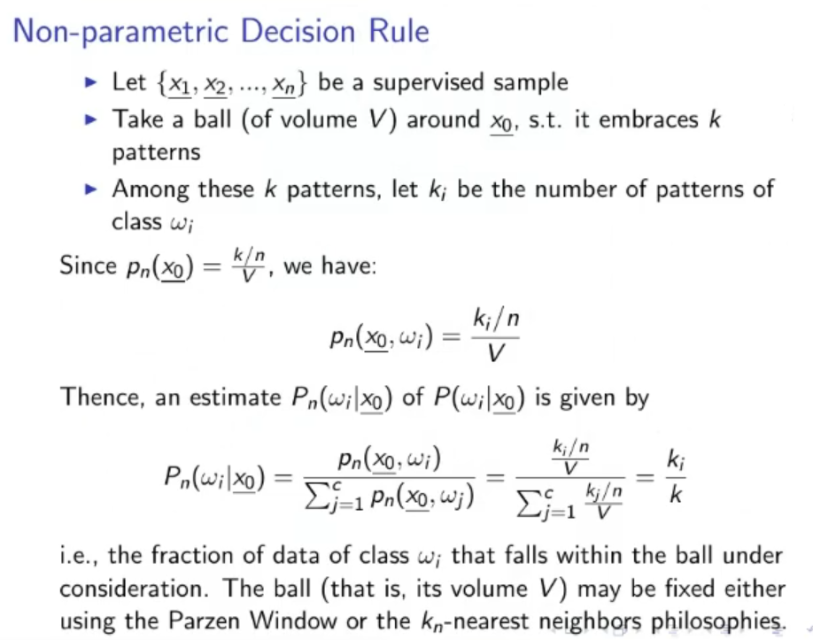
Non-Parametric Decision Rule*:

• $\{\underline{x_1},\underline{x_2},\dots ,\underline{x_n}\}$ : be a supervised sample.
• $V$ : volume of the ball embracing $k$ patterns.
• $k_i$ : how many patterns among the $k$ pattern, belong to class ${\omega }_i$.

⇒ Since $p_n(\underline{x_0})=\frac{k}{nV}$ we will have that the probability that $x_0$ will belong to class ${\omega }_i$ is:

$$p_n(\underline{x_0},{\omega }_i)=\frac{k_i}{nV}$$

⇒ Hence an estimate $P_n({\omega }_i|\underline{x_0})$ of $P({\omega }_i|\underline{x_0})$ is given by:

$$P_n({\omega }_i|\underline{x_0})=\frac{p_n(\underline{x_0},{\omega }_i)}{{\sum }_{j=1}^c{p}_n(\underline{x_0},{\omega }_j)}=\frac{\frac{k_i}{nV}}{{\sum }_{j=1}^c\frac{k_j}{nV}}=\frac{k_i}{k}$$

Where:

• ${\sum }_{j=1}^c{p}_n(\underline{x_0},{\omega }_j)$ : means the probability that $\underline{x_0}$ will belong to one of the classes $k_j$, so it is equal to $\frac{k}{nV}$.

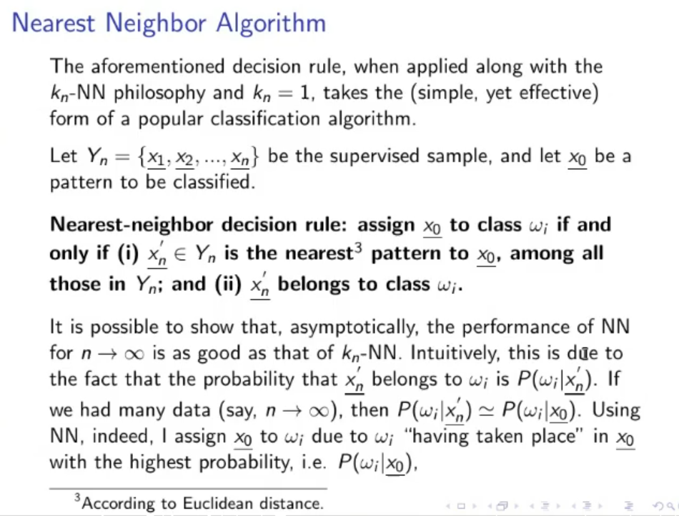
Nearest Neighbour Decision Rule: Assign $\underline{x_0}$ to class ${\omega }_i$ if and only if:

1. $\underline{x_n^{\prime }}\in Y_n$ is the nearest (according to Euclidean Distance) to $\underline{x_0}$, among all those in $Y_n$.
2. $\underline{x_n^{\prime }}$ belongs to class ${\omega }_i$.

Where:

• $Y_n=\{\underline{x_1},\underline{x_2},\dots ,\underline{x_n}\}$ : supervised sample.
• $\underline{x_0}$ : pattern to be classified.

ALGORITHM: Search for the closest element of $\underline{x_0}$ in $Y_n$, let’s say $x_i$ that belong to class ${\omega }_i$. Then we will classify $x_0$ with the class ${\omega }_i$.

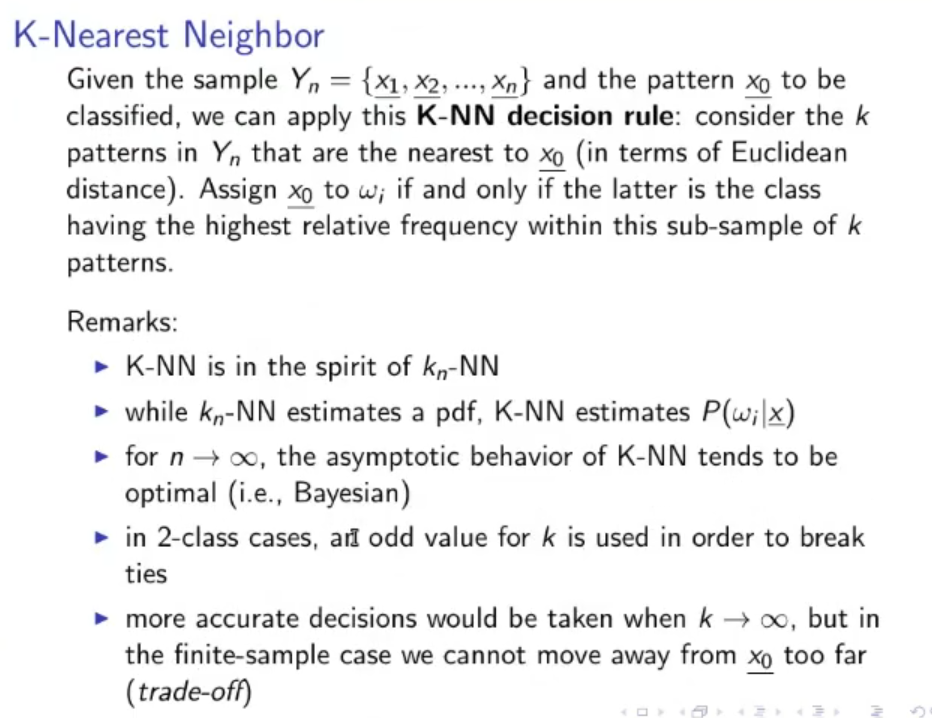
K-Nearest Neighbor (K-NN): To not be confused with $k_n$-NN ($k_n$-Nearest Neighbour)

• $Y_n=\{\underline{x_1},\underline{x_2},\dots ,\underline{x_n}\}$ : supervised sample.
• $\underline{x_0}$ : pattern to be classified

⇒ Algorithm:

1. Consider the $k$ patterns in $Y_n$ that are closer to $\underline{x_0}$ in term of Euclidean distance)
2. $\underline{x_0}$ belongs to ${\omega }_i$, where ${\omega }_i$ is the class with the highest relative frequency within the $k$ sample taken into consideration.

NOTE: While $k_n$-NN estimates a pdf, the K-NN algorithm estimates $P({\omega }_i|\underline{x})$

• For $n\to \infty$, the asymptotic behaviour of the K-NN tends to be optimal (~ex.: Bayesian)
• In $K=2$ cases or more generally, in cases where 2 or more classes have the same relative frequency we can expand the neighbour (increasing K) until there is only one class that has higher relative frequency with respect to the others.
• The higher the value of $K$ the more accurate are the decisions taken, but it will take more time (trade-off)

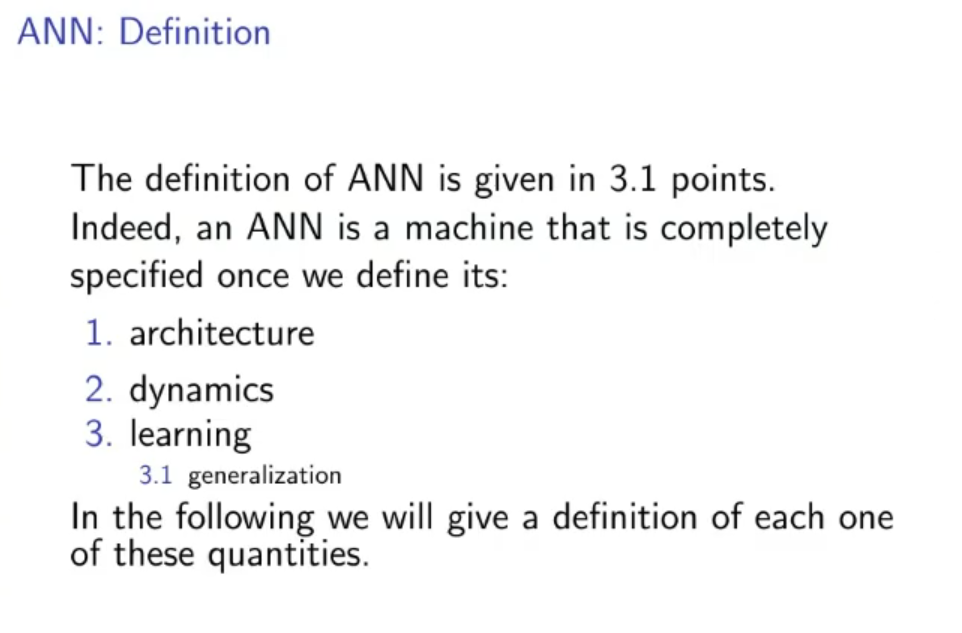
Definition of an ANN (Artificial Neural Networks): An ANN is completely specified once we define its:

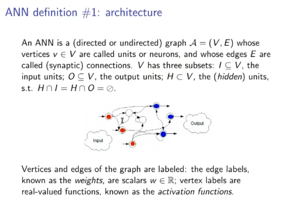
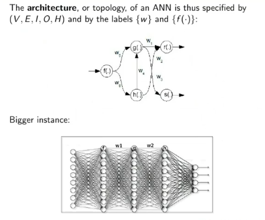
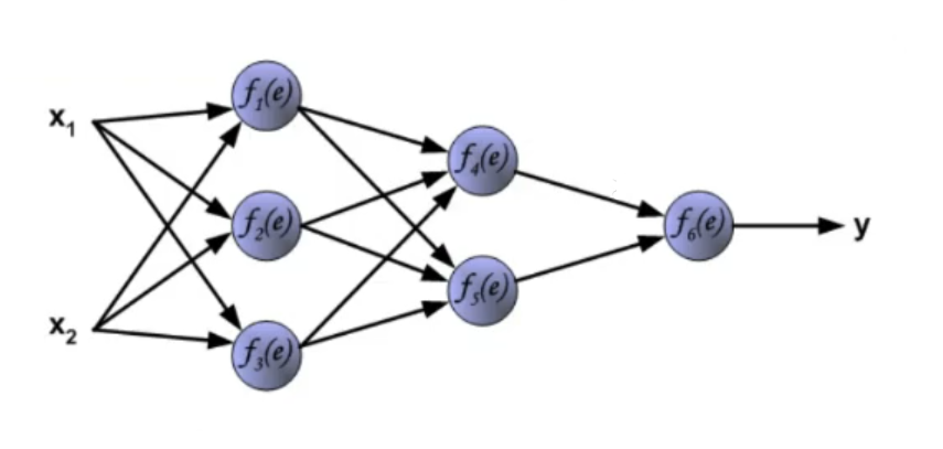
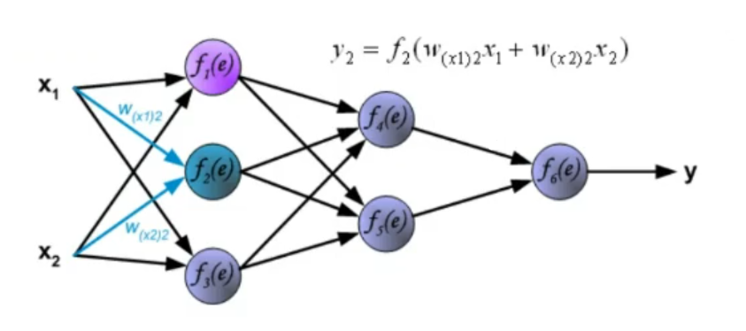
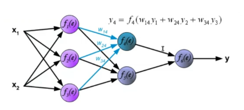
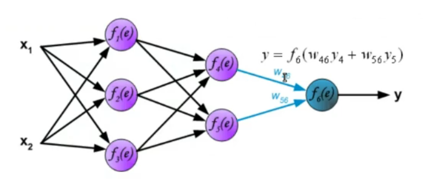
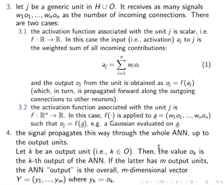
1. Architecture: An ANN is a directed or un-directed graph where each node (or vertices) is called a neuron and each arch (or edge) is called a synaptic connection, it has three subset: the input units, the output units and the hidden units. ⇒ For each node we can define an activation function ⇒ While for each arch we can define its weight. An architecture is completely defined with: Vertices, Edges, Input Units, Output Units, Hidden Units, Weights and Activation Functions.

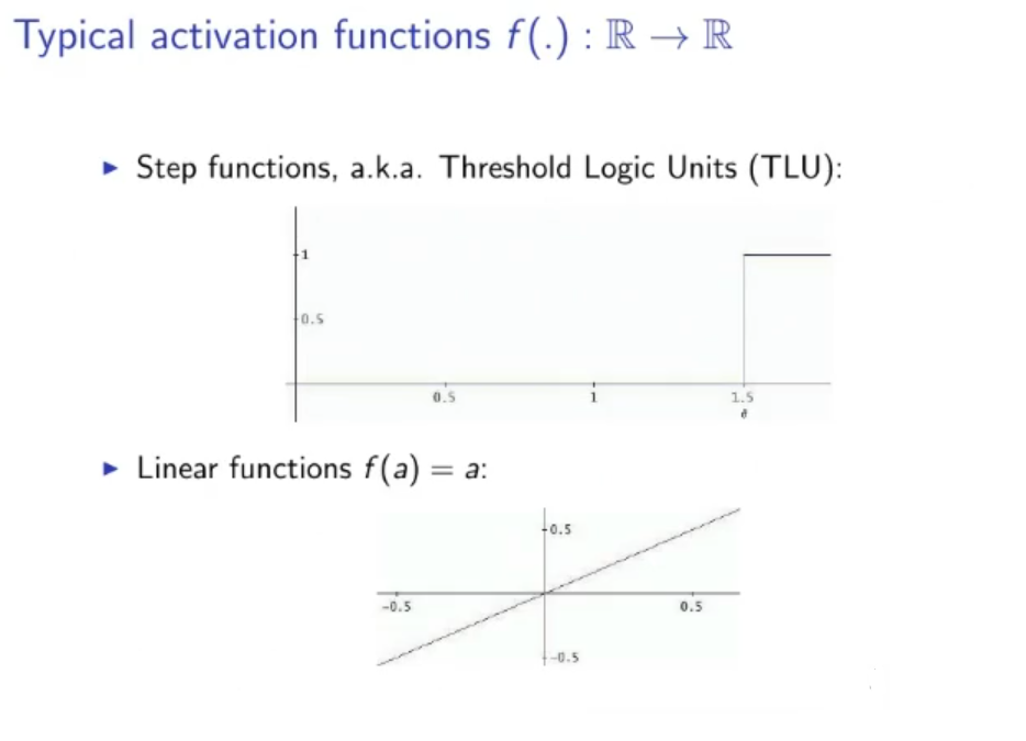
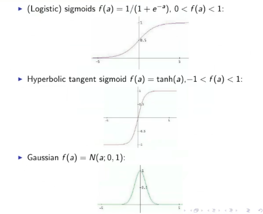
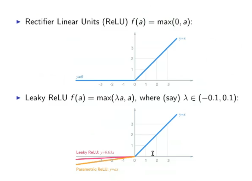
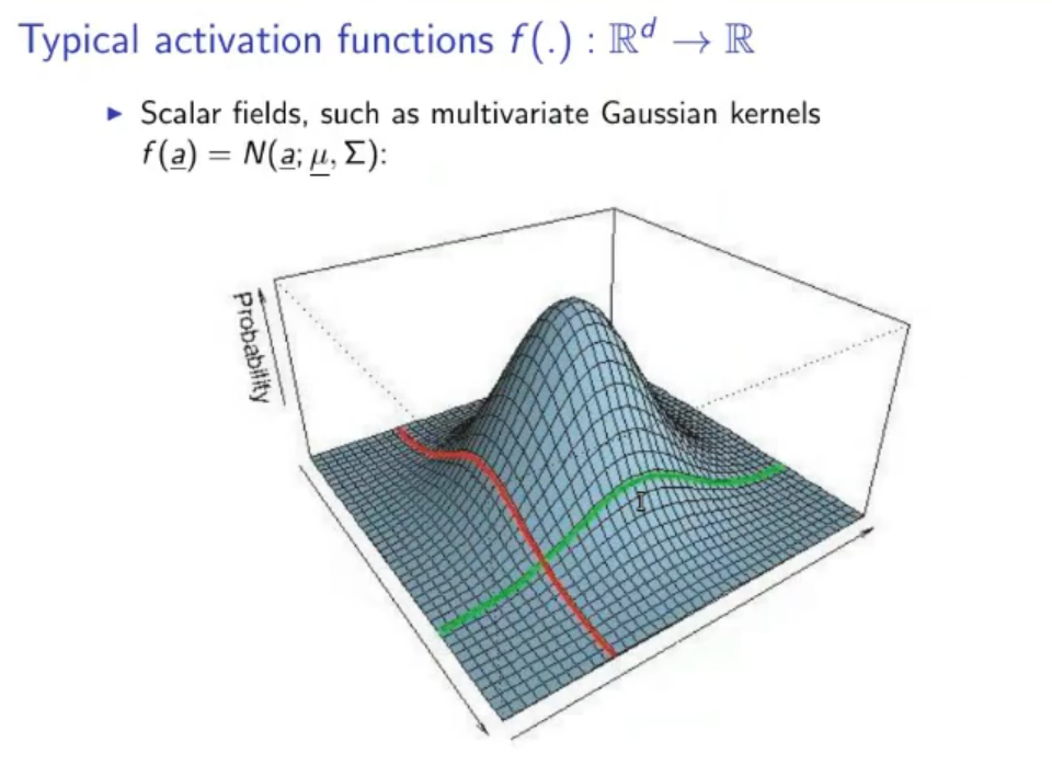
1.1. Typical Activation Functions: ⇒ Step function or TLU (Threshold Logic Units): $f(a)=1(a),f(a)\in [0,1]$ ⇒ Linear Function: $f(a)=a,f(a)\in \mathbb{R}$ ⇒ Sigmoid function: $f(a)=\frac{1}{1+e^{-a}},f(a)\in [0,1]$ ⇒ Hyperbolic tangent sigmoid: $f(a)=\tanh (a),f(a)\in [-1,1]$ ⇒ Gaussian: $f(a)=N(a;\mu ,{\sigma }^2),f(a)\in [0,1]$ ⇒ ReLU (Rectifier Linear Units): $f(a)=\max (0,a),f(a)\in [0,+\infty ]$ ⇒ Leaky ReLU: $f(a)=\max (\lambda a,a),\text{where}\lambda \in [-0.1,0.1]$

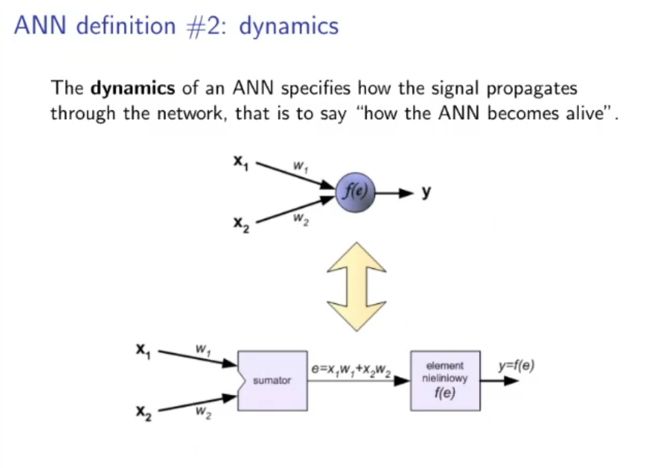
2. Dynamics: How the signal propagates. The dynamics of an ANN represent how the input data goes from start to end (how it “propagates”), we need to define how the weights interact with the data after they are processed by the activation function. ~Ex.: Let’s take $d$ input data $(x_1,x_2,\dots ,x_d)$ these data will not have any transformation in the input (even this part can be changed), then they will pass through a first hidden layer where for each node the activation function will be something like:

$$\begin{array}{rl}& a_j=\sum _{i=1}^d{w}_i{o}_i\\ & z_j=\sigma \left(a_j\right)\end{array}$$

Where: $o_i$ : old layers (from $1$ to $d$) (in this case the input) $z_j$ : node $j$ belonging to the new layer (in this case the hidden layer) $\sigma$ : sigmoid function (our chosen activation function)

~Ex.:

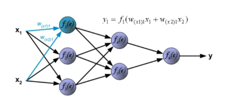
This process is then repeated until the signal reaches the output layer.

Also the dynamics also define the clock (time trigger) of the ANN, which depends on its family of networks.

NOTE: The ANN topology specifies the hardware architecture, the value of the weights it’s the software, while the ANN dynamics (the living machine) represents the running process.

3. Learning: The ANN learns from the examples contained in the training set $\tau =\{\underline{z_1},\underline{z_2},\dots ,\underline{z_n}\}$ which is a continuous-valued data sample drawn from an underlying multivariate pdf. Main learning setups: ⇒ Supervised Learning: $\tau =\{(\underline{x_1},\underline{y_1}),\dots ,(\underline{x_n},\underline{y_n})\}$ ⇒ Unsupervised Learning: $\tau =\{\underline{x_1},\dots ,\underline{x_n}\}$ ⇒ Semi-Supervised Learning: $\tau =\{(\underline{x_1},\underline{y_1}),\dots ,(\underline{x_n},\underline{y_n}),\underline{x_{n+1}},\dots ,\underline{x_{n+m}}\}$ $n$ training data are supervised, they are a set of input $x_i$ and output $y_i$, while $m$ data are unsupervised, we know the input $x_j$ but not its output ⇒ Reinforcement Learning: $\tau =\{\underline{x_1},\underline{x_2},\dots ,(\underline{x_t},\underline{y_t}),\underline{x_{t+1}},\dots \}$ Where a reinforcement signal $y_t$ either a penalty or a reward is given every now and then.

3.1. Generalization: Learning is a process of progressive modification of the connection weights, aimed at inferring the (universal) law underlying the data. Far from being a mere memorization of the data, the laws learned this way are expected to generalize new data, previously unseen, this is called generalization capability.

---

Original Files:

---

---