PF Algorithm

Explanation of the Algorithm

~Example taken from Youtube

Given the map of a building an a robot with a laser sensor we want to estimate the position of the robot.

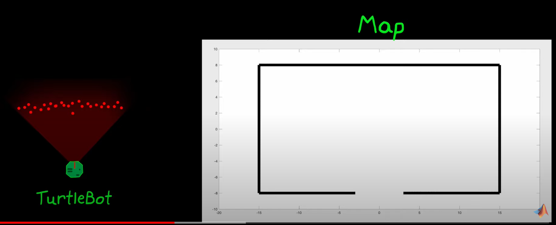
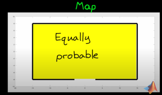
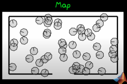
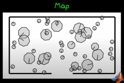
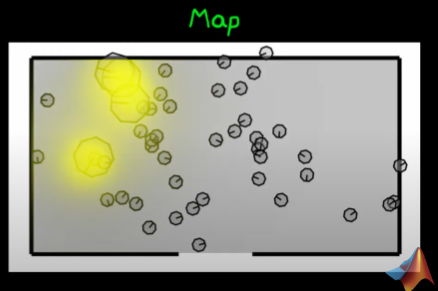
1. The robot could be anywhere on the map, to do this I take a finite set of randomly taken bot (random position, random orientation) and put the in a simulated map:
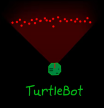
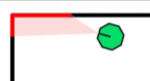
2. I take the measurement of the bot:
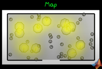
3. I estimate where the robot could be (considering a possible error in the measurements) and highlight the more probable simulated robots: New simulated pdf:
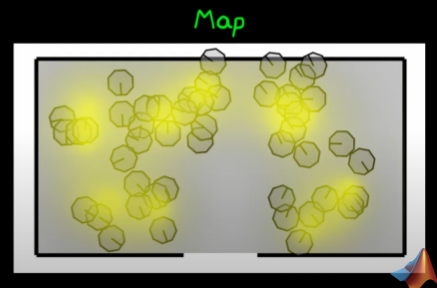
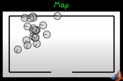
4. Using the new pdf i re-randomize the simulated robots and their positions:
5. I repeat the process:

• Measurement.
• Estimation of pdf.
• Randomize new simulated robots.

This Algorithm is also known as MCL (Monte Carlo Localization). A variant of this algorithm, the AMCL ( Adaptive Monte Carlo Localization) reduces the number of simulated robots at each iteration, to speed up the algorithm, it’s a little less precise, but much more quick.

---

Algorithm

0. Initialization:

• We need to know the pdf: $f_x$, $f_w$, $f_v$ as well as the functions $f$ and $h$.

1. Generate $X^{(i)}$ $i=1,\dots ,p$ particles according to the distribution $f_x(x(t)|Y^t)$
2. Generate $W^{(i)}$ $i=1,\dots ,p$ particles according to the distribution $f_w(w(t))$
3. $X_{t+1}^{(i)}=f\left(X_t^{(i)},u(t),W_t^{(i)}\right)$ Which are the particles rappresentative of the distribution $f_x(x(t+1)|Y^{t+1})$
4. $f_z(z(t)|X_t^{(i)})=f_v\left(z(t)-h(X_t^{(i)})\right)$
5. Generate a set of $p$ weights $q_i$ such that:

$$\begin{array}{rl}& q_i=\frac{f_z(y(t)|X_t^{(i)})}{{\sum }_{j=1}^p{f}_z(z(t)|X_t^{(j)})}i=1,\dots ,p\\ & q_i\in \left[0,1\right]\\ & \sum _{i=1}^p{q}_i=1\end{array}$$

6. Create a new discrete distribution function $f_x$ such that:

$$\mathbb{P}\left\{x=X_t^{(i)}\right\}=q_{i}i=1,\dots ,p$$

7. Using the new $f_x$ restart from point (1.)