-
Basic Knowledge and Notation:
-
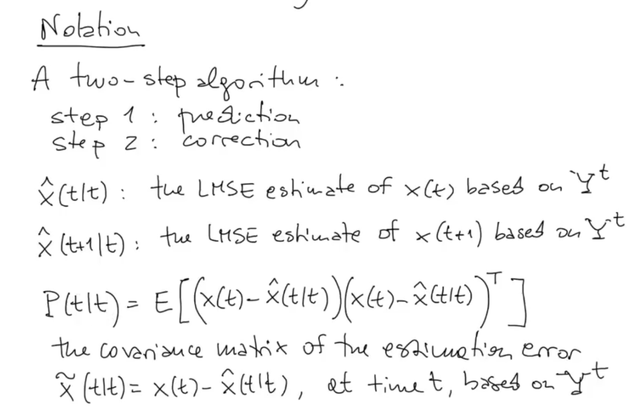
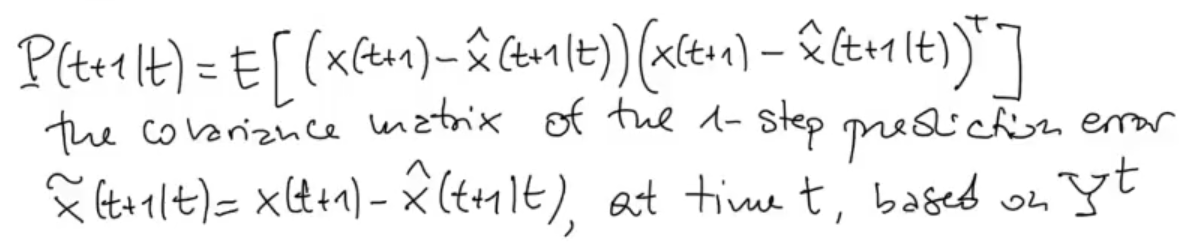
PREDICTION STEP:
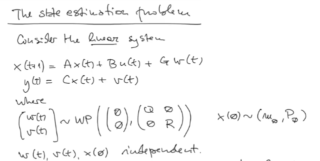
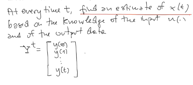
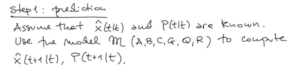 Define the problem
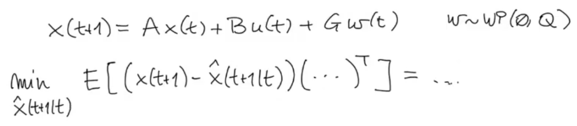 We could also write as our objective function the LMSE (Least Mean Square Error), but it will bring the exact same result.
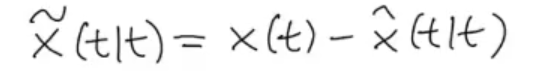
For simplicity we will define:
We could also write as our objective function the LMSE (Least Mean Square Error), but it will bring the exact same result.
For simplicity we will define:
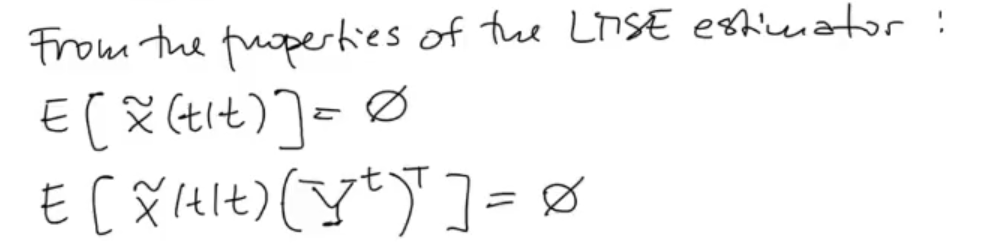
 And since we are searching for the LMSE estimator (or similar, the result will still be the LSME estimator):
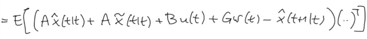
 We substitute
 We use the previous definition of :
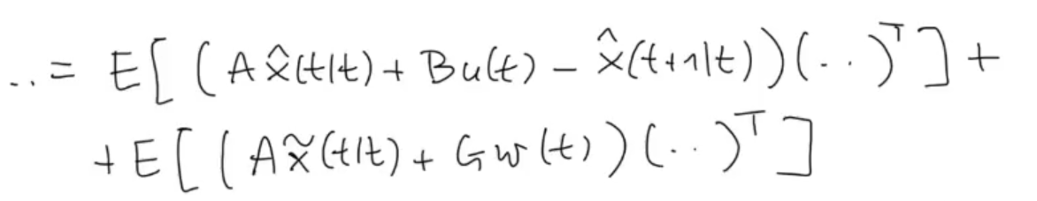
 We remove the uncorrelated part:
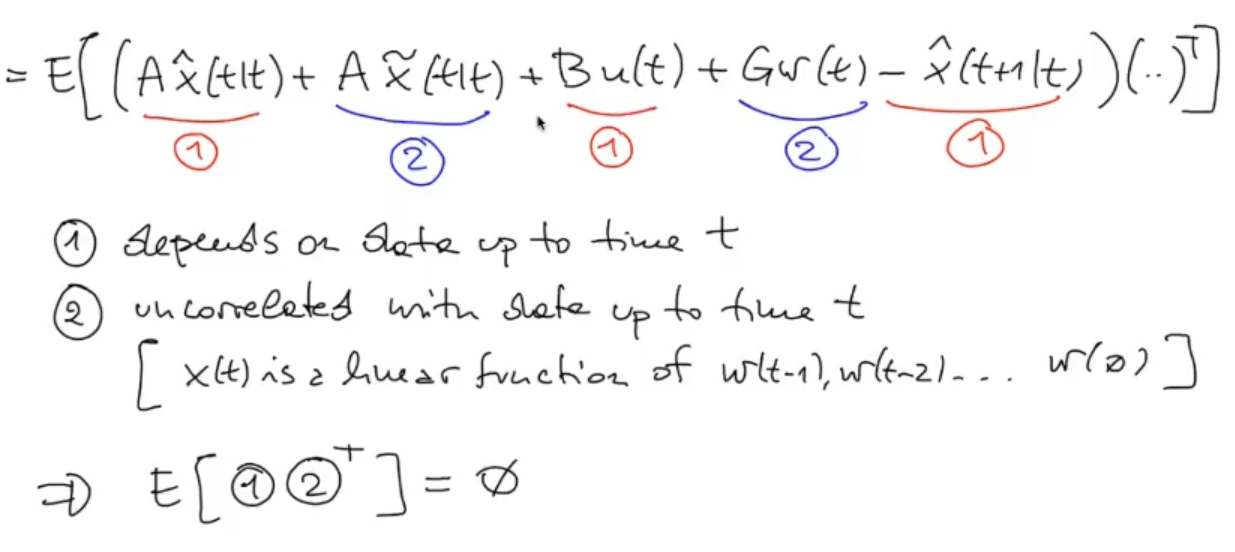 So only the products of (1)(1) and (2)(2) remains:
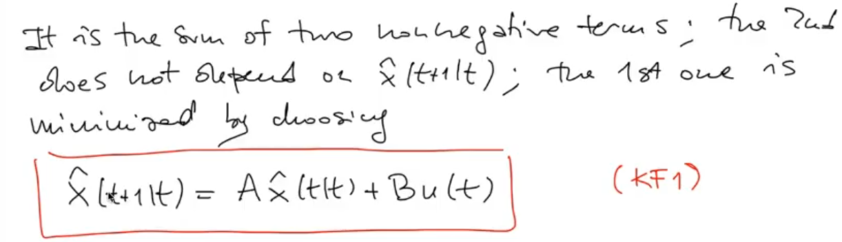
 The variance is always positive, so by choosing such that the first component is is the best possible result, after all the second component only depends on which I cannot change.
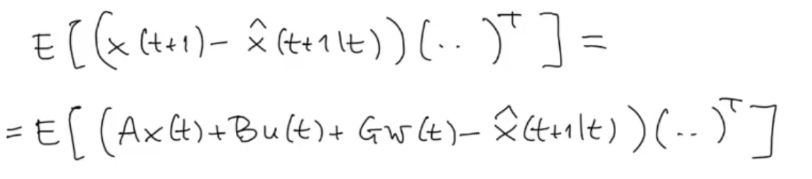
 Now let’s see how changes, starting from its definition as the covariance matrix of the error on the prediction :
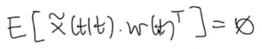
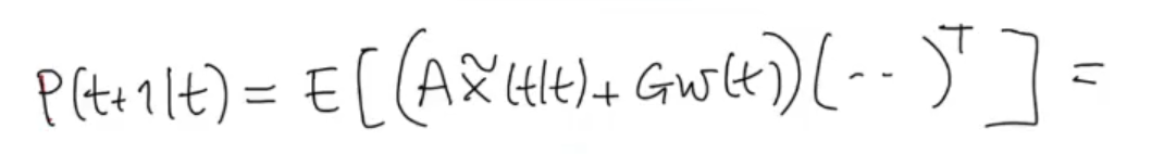 Knowing that since is a white process:
 Then:
Then:
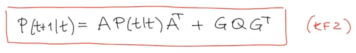
 We can rewrite it as we have already seen as the Discrete Lyapunov Equation:
-
CORRECTION STEP:
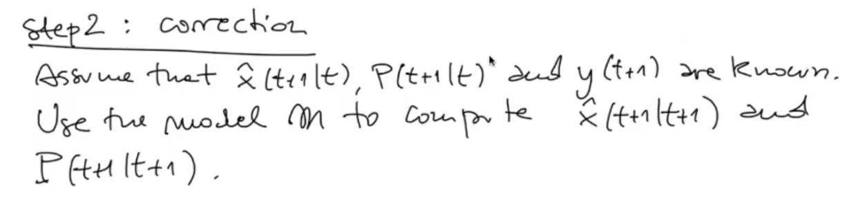 Define the problem:
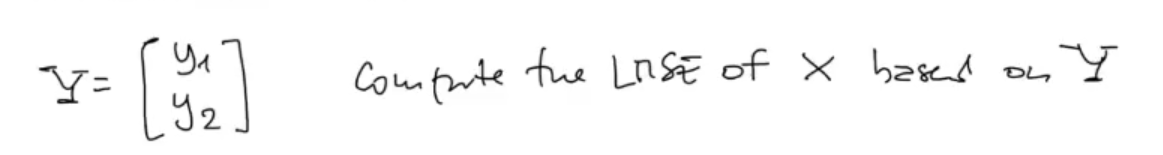 Where:
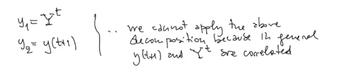
- is the measurement vector obtained at time
- is the measurement vector obtained at time
We already know the solution of this problem:
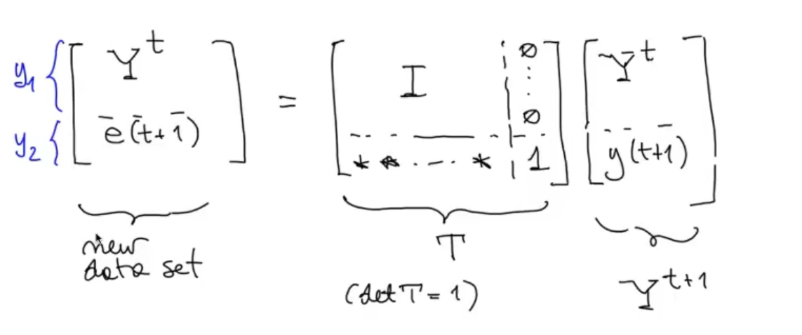
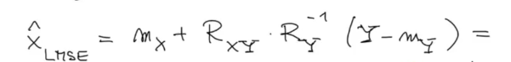 Now we need to use all the information we got:
We know that is divided in 2 parts and , so:
Now we need to use all the information we got:
We know that is divided in 2 parts and , so:
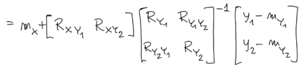 We now make a strong assumption, we say that and are uncorrelated, unfortunately in most cases this is not the case:
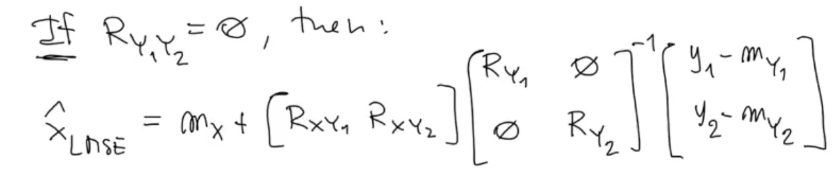 The inverse of a diagonal matrix is:
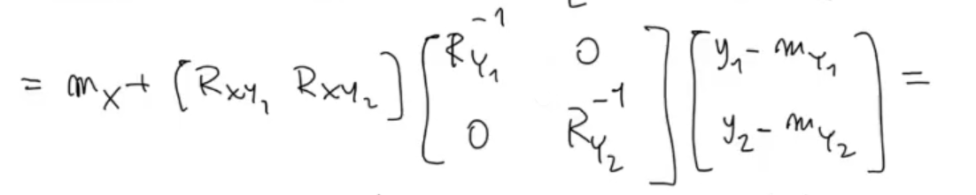 We solve the matrix product:
 Here we can say somenting:
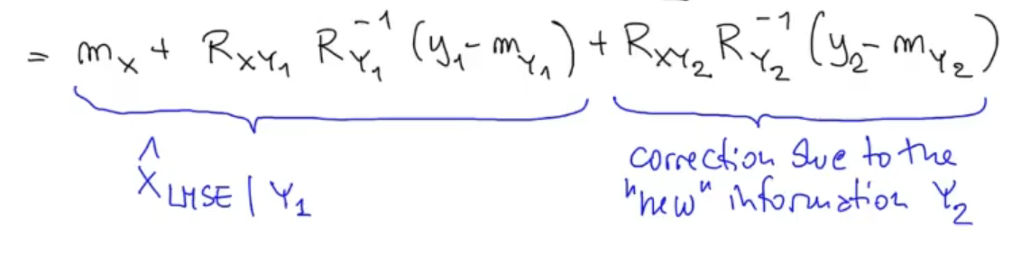 But unfortunately, this works only if and are uncorrelated:
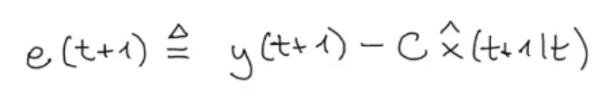
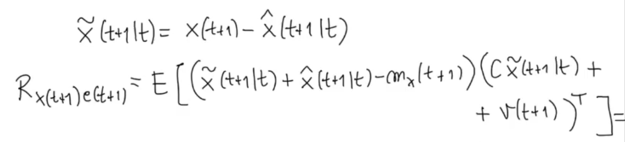
Let’s now define the so called Innovation Process:
 The idea behind it is that we want to correct using only the new information contained in , so ignore from the old information, already seen in .
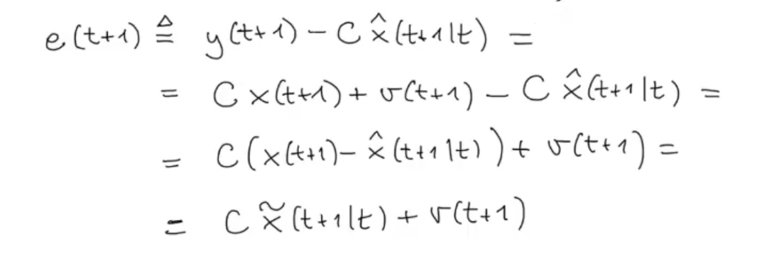
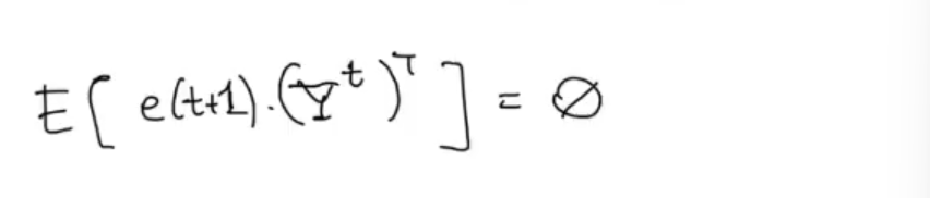
We can see the innovation process as the error of what the sensor measured (so the “almost” ground truth, whit an added noise ) and what our model predicted:
Doing some simple substitutions we have that the innovation process is equal to:
It also has some nice properties:
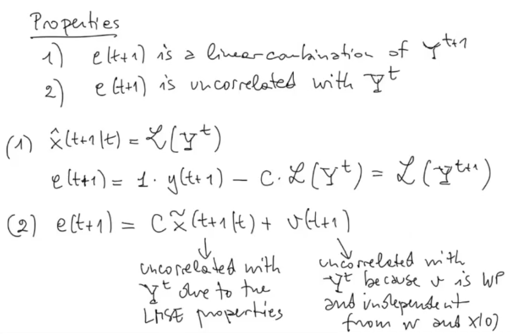 We say that is a linear combination of , because we know that the mathematical model is linear and as we can see from it is a prediction of that depends on the measurement up to time , ergo it’s a linear combination of .
Now we can define the “update” process as:
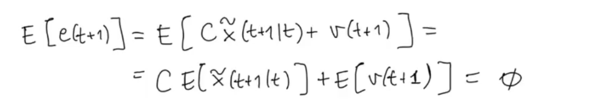
Since is uncorrelated with :
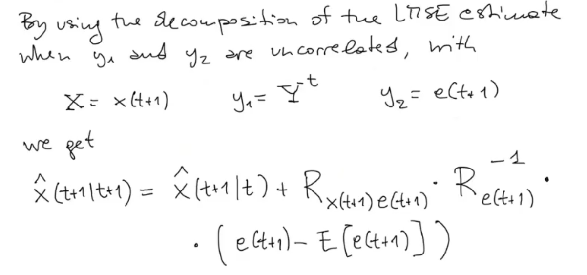
Where:
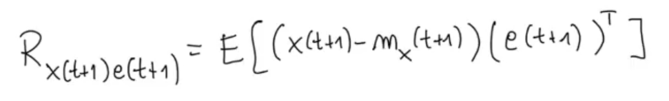
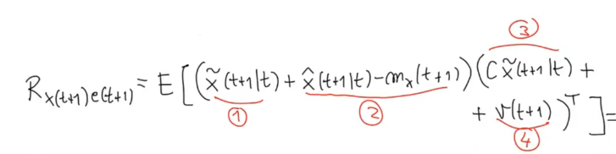
 By the definition of covariance:
 Like we did previously:
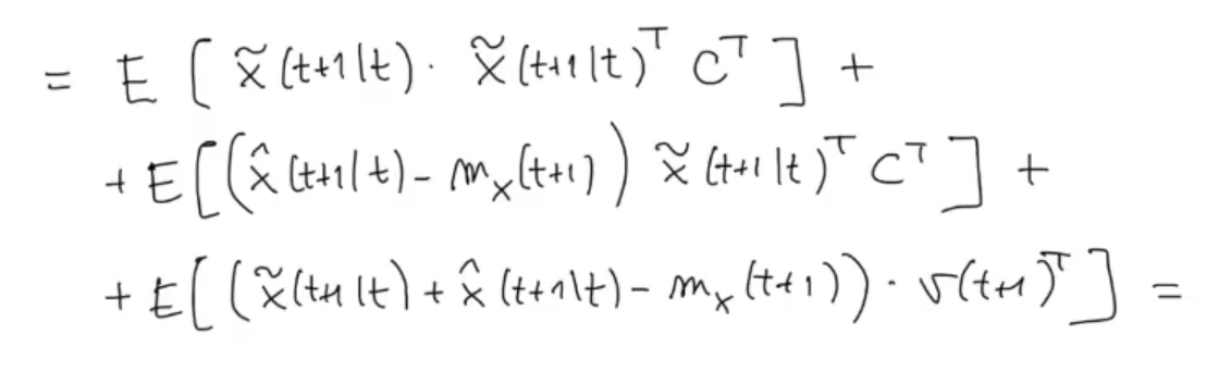
 We study how the double product interact with each other:
 And we have that:
 We can “delete” the last two terms:
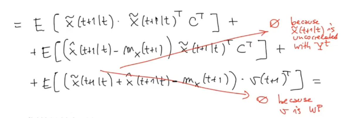 And we have that is equal to:

We calculate also the variance of :
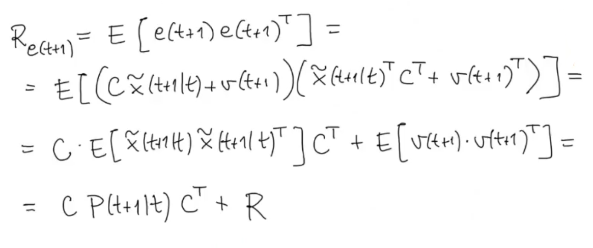 (Like before we can simplify because is a White Process)
So we can say that
is equivalent to:
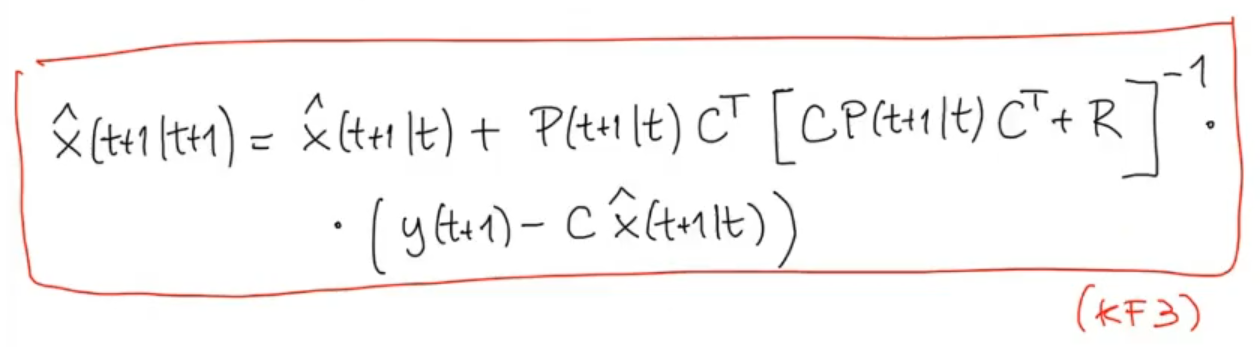
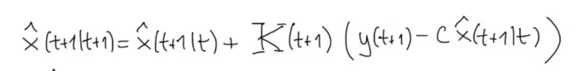
We define the Kalman Gain:
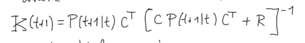
Such that:
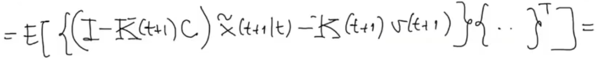
We have seen how evolves, now let’s see how evolves, starting as always by its definition:
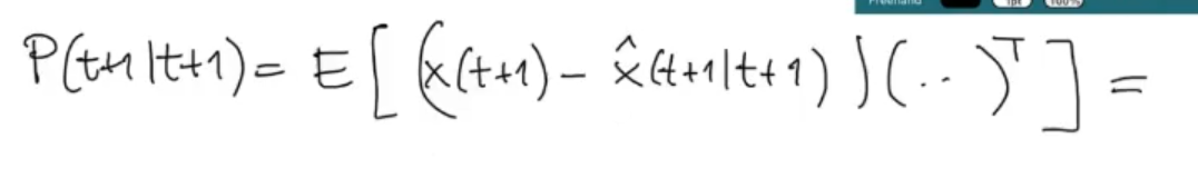 We substitute the just found :
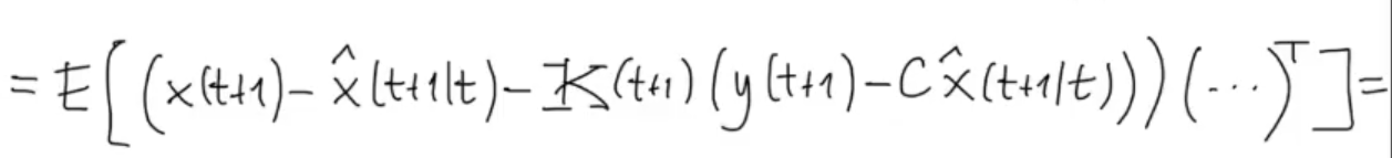 Then we substitute , and :
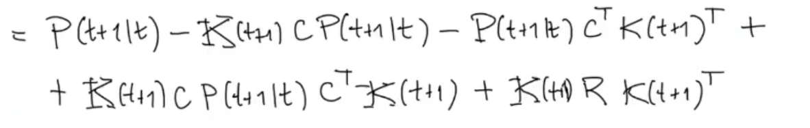
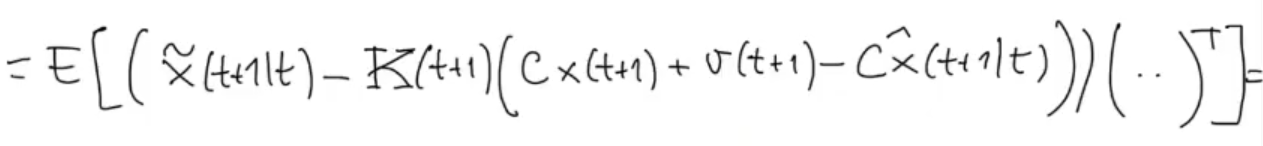 Simple multiplication, and substitution for
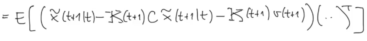 We group :
 Like before:
- The covariance of something (different from ) multiplied by is zero since is a White Process.
- The variance of is , as defined in the formulation of the problem.
- The covariance of is , from the definition of
- Also note that , and are not stochastic.

We can simplify the formula, first we develop the matrix multiplication:
 Then we simplify:
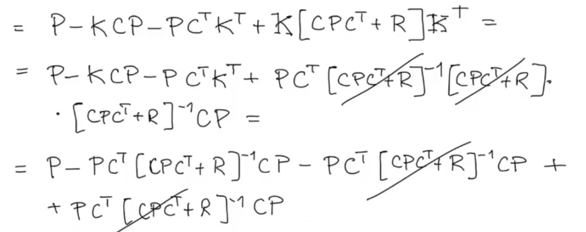
Finally we obtain the last formula for the KF algorithm:
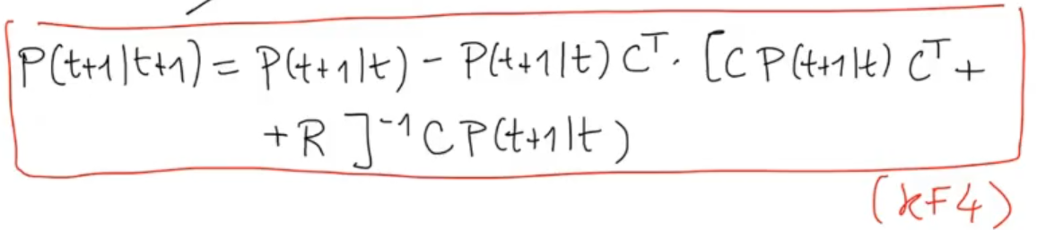 Can also be written as:
 3. Iterate