C-D EKF Algorithm

Algorithm

0. Initialization:
1. PREDICTION STEP:

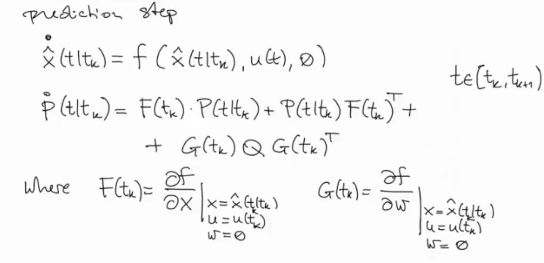
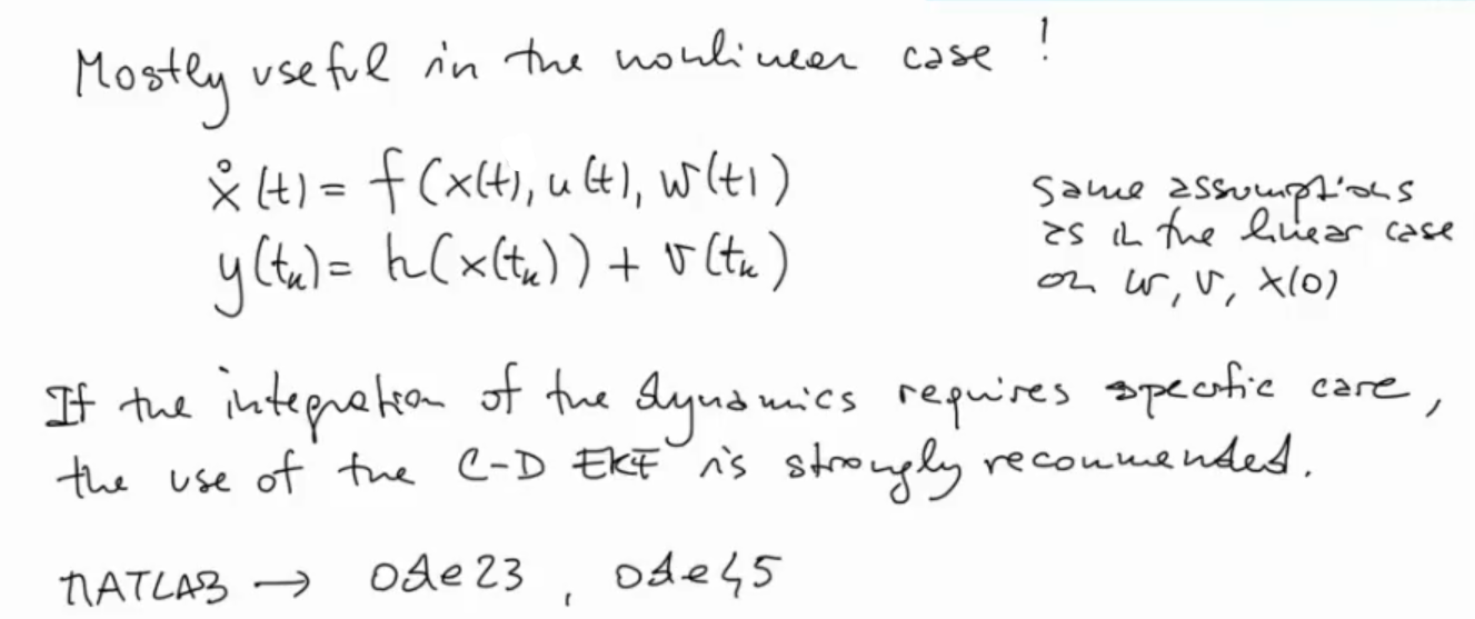
NOTE: In the first equation of the prediction step we are required to solve a differential equation, to do this we can use the functions ode23 and ode45 in MATLAB, which will solve the differential equations (at each loop) numerically.

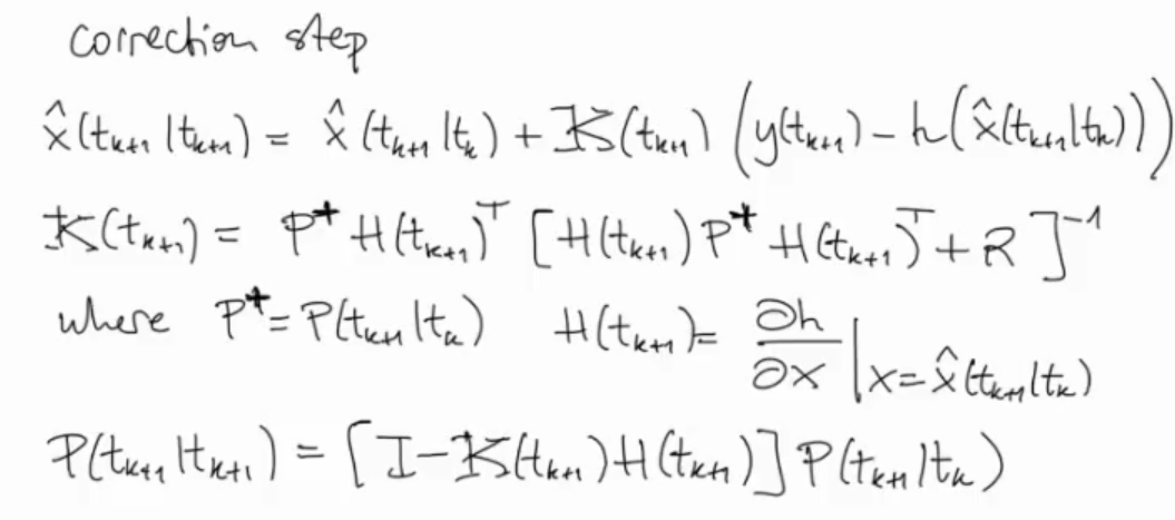
2. CORRECTION STEP:
3. Iterate, from point (1.)

---

~Example ‘Differences from the EKF and C-D EKF Solutions’

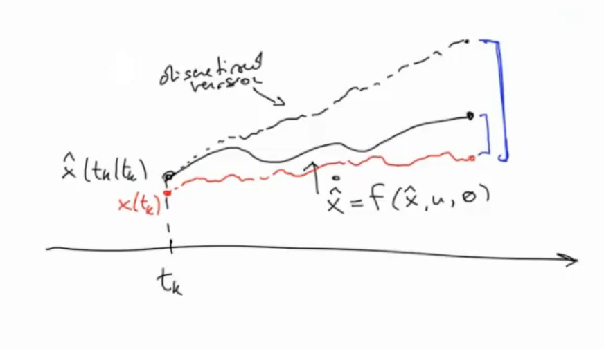
• The discretized version (dashed black line) is obtained using the EKF algorithm
• The continuous version (black line) is obtained using the C-D EKF algorithm
• While in red we can see the true state $x(t_k)$ of the system.